Demagnified Solutions#
Overview#
When fitting a lens model using a pixelized source reconstruction, it is common for unphysical and inaccurate lens models to be estimated.
This is due to demagnified source reconstructions, where the source is reconstructed as the lensed source galaxy (without any lensing):


What has happened above is that the mass model has gone to an extremely low mass solution, such that essentially no ray-tracing occurs. The best source reconstruction to fit the data is therefore one where the source is reconstructed to look exactly like the observed lensed source.
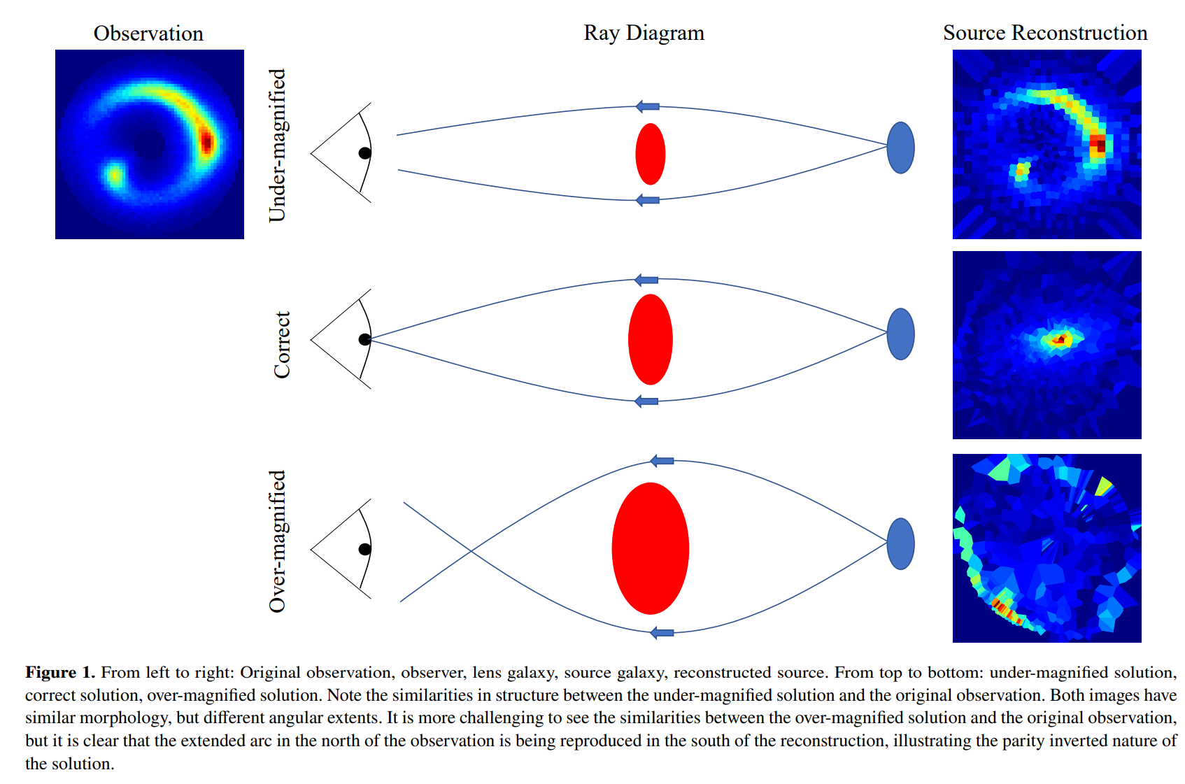
In fact, there are two variants of these unwanted systematic solutions, with the second variant corresponding to mass models with too much mass, such that the ray-tracing inverts in on itself.
The following schematic is from the paper Maresca et al 2021 (https://arxiv.org/abs/2012.04665) and illustrates this beautifully:
The source reconstructions and model-fits of these solutions are also illustrated by Maresca et al 2021:
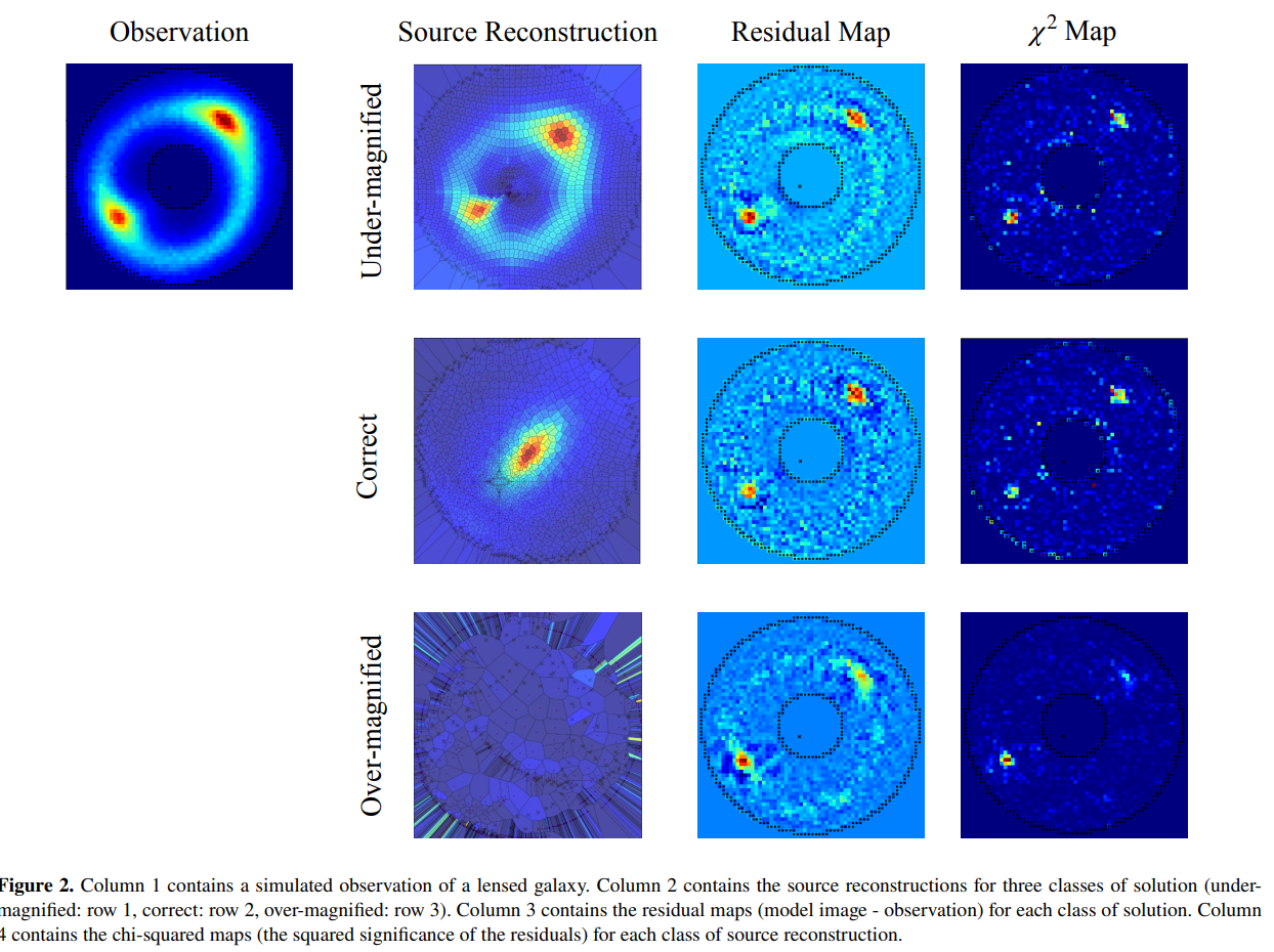
The demagnified solutions are not as high likelihood as the physical and accurate mass model shown in the central row of the figure above. However, the demagnified solutions occupy a much greater volume of non-linear parameter space.
This means that when we fit a lens model, it is highly probable that all solutions correspond to demagnified solutions, such that the non-linear search converges on these solutions and never samples the accurate physical mass model.
Solution#
To prevent a non-linear search from inferring these unwanted solutions PyAutoLens penalizes the likelihood via a position thresholding term.
First, we specify the locations of the lensed source’s multiple images, which the example code below does:
positions = al.Grid2DIrregular(
    grid=[(0.4, 1.6), (1.58, -0.35), (-0.43, -1.59), (-1.45, 0.2)]
)
Here is where the multiple images appear for an example strong lens, where multiple images are drawn on with black stars:

The autolens_workspace also includes a Graphical User Interface for drawing lensed source positions via
mouse click (https://github.com/PyAutoLabs/autolens_workspace/blob/main/scripts/imaging/preprocess/gui/positions.py).
Next, we create PositionsLH object, which has an input threshold.
This requires that a mass model traces the multiple image positions specified above within the threshold
value (e.g. 0.5”) of one another in the source-plane. If this criteria is not met, a large penalty term is
applied to likelihood that massively reduces the overall likelihood. This penalty is larger if the positions
trace further from one another.
This ensures the unphysical solutions that produce demagnified solutions have a much lower likelihood that the
physical solutions we desire. Furthermore, the penalty term reduces as the image-plane multiple image positions
trace closer in the source-plane, ensuring the non-linear search (e.g. Dynesty) converges towards an accurate mass
model. It does this very fast, as ray-tracing just a few multiple image positions is computationally cheap.
If the positions do trace within the threshold no penalty is applied.
The penalty term is created and passed to an Analysis object as follows:
positions_likelihood = al.PositionsLH(positions=positions, threshold=0.3)

analysis = al.AnalysisImaging(
    dataset=dataset, positions_likelihood_list=[positions_likelihood]
)
The threshold of 0.5” is large. For an accurate lens model we would anticipate the positions trace within < 0.01” of one another. However, we only want the threshold to aid the non-linear with the choice of mass model in the initial fit and remove demagnified solutions.
Auto Position Updates#
There are a number of downsides to having to input the multiple images positions manually:
For large lens samples this could take a lot of time.
For complex sources, it can be unclear which brightness peaks in the image-plane lensed source correspond to the same emission in the source-plane.
PyAutoLens allows the positions and threshold to be computed if a model for the lens mass is available.
This is the case for lens modeling pipelines which use PyAutoLens’s search chaining functionality, because the early fits in these pipelines fit a parametric source model which does not suffer these demagnified solutions.
If we have a result from a previous search, which contains a mass model for the lens galaxy and a light model
for the source (the centre of which is used to compute the multiple image positions) we can compute a new
set of multiple image positions from this result:
result.image_plane_multiple_image_positions
We can also compute a threshold from the result, where this threshold value corresponds to the maximum separation
of the result.image_plane_multiple_image_positions computed above but ray traced to the source-plane using
the result’s maximum likelihood mass model.
result.positions_threshold_from(factor=2.0, minimum_threshold=0.3)
The factor input is a value that the computed threshold is multiplied by. For example, if a threshold of
0.1” is computed, the returned value above for factor=2.0 will be 0.2”.
The minimum_threshold is the lowest number the function return will reutnr. Above, if a threshold of 0.1”
is computed, the function will return 0.3” because minimum_threshold==0.3.
These inputs are useful when using function to set the threshold in a new fit of a search chaining pipeline, as
it allows us to make sure we do set too small a threshold that we remove genuinely physically mass models.
For writing search chaining pipelines, a convenience method is available in the result which returns directly a
PositionsLH object:
result_1.positions_likelihood_from(
    factor=3.0, minimum_threshold=0.2
)
This is often used to set up new Analysis objects with a positions penalty concisely:
analysis = al.AnalysisImaging(
    dataset=dataset,
    positions_likelihood_list=[result_1.positions_likelihood_from(
        factor=3.0, minimum_threshold=0.2
    )],
)
Multiple Source Plane Systems#
A double source plane system is a lens system where there are multiple source-planes at different redshifts, meaning that incuding the image-plane there are at least 3 planes.
The PositionsLH class can have a plane_redshift input, which specifies the redshift of the source-plane
the positions are ray-traced to.
Multiple PositionsLH objects can be passed to the Analysis object, which then applies the penalty term to
both source-planes independently such that a double source-plane system can be fitted with the penalty based likelihood
functionality.
positions_likelihood_source_plane_0 = al.PositionsLH(positions=positions, threshold=0.3, plane_redshift=1.0)
positions_likelihood_source_plane_1 = al.PositionsLH(positions=positions, threshold=0.3, plane_redshift=2.0)

analysis = al.AnalysisImaging(
    dataset=dataset, positions_likelihood_list=
        [
            positions_likelihood_source_plane_0,
            positions_likelihood_source_plane_1
        ]
)
To set up an Analysis object with multiple PositionsLH objects from a result, each positions likelihood is
computed from the result for each plane_redshift:
analysis = al.AnalysisImaging(
    dataset=dataset,
    positions_likelihood_list=[
        source_lp_result.positions_likelihood_from(
            factor=3.0, minimum_threshold=0.2, plane_redshift=source_lp_result.instance.galaxies.source_1.redshift,
        ),
        source_lp_result.positions_likelihood_from(
            factor=3.0, minimum_threshold=0.2, plane_redshift=source_lp_result.instance.galaxies.source_2.redshift,
        )
    ],
)