Model Cookbook#

The model cookbook provides a concise reference to lens model composition tools, specifically the Model and Collection objects.

Examples using different PyAutoLens API’s for model composition are provided, which produce more concise and readable code for different use-cases.

Simple Lens Model#

A simple lens model has a lens galaxy with a linear Sersic light profile, Isothermal mass profile and source galaxy with a linear Sersic light profile:

# Lens:

bulge = af.Model(al.lp_linear.Sersic)
mass = af.Model(al.mp.Isothermal)

lens = af.Model(
    al.Galaxy,
    redshift=0.5,
    bulge=bulge,
    mass=mass,
)

# Source:

source = af.Model(al.Galaxy, redshift=1.0, bulge=al.lp_linear.SersicCore)

# Overall Lens Model:

model = af.Collection(galaxies=af.Collection(lens=lens, source=source))

The redshifts in the above model are used to determine which galaxy is the lens and which is the source.

The model total_free_parameters attribute tells us the total number of free parameters (which are fitted for via a non-linear search), which in this case is 17 (6 from the lens Sersic, 5 from the lens Isothermal and 6 from the source SersicCore). The intensity of each linear light profile is not one of them: it is solved for by the inversion during every likelihood evaluation.

print(f"Model Total Free Parameters = {model.total_free_parameters}")

If we print the info attribute of the model we get information on all of the parameters and their priors.

print(model.info)

This gives the following output:

Total Free Parameters = 17

model                                                                           Collection (N=17)
    galaxies                                                                    Collection (N=17)
        lens                                                                    Galaxy (N=11)
            bulge                                                               Sersic (N=6)
            mass                                                                Isothermal (N=5)
        source                                                                  Galaxy (N=6)
            bulge                                                               SersicCore (N=6)

galaxies
    lens
        redshift                                                                0.5
        bulge
            centre
                centre_0                                                        GaussianPrior [0], mean = 0.0, sigma = 0.3
                centre_1                                                        GaussianPrior [1], mean = 0.0, sigma = 0.3
            ell_comps
                ell_comps_0                                                     TruncatedGaussianPrior [2], mean = 0.0, sigma = 0.3, lower_limit = -1.0, upper_limit = 1.0
                ell_comps_1                                                     TruncatedGaussianPrior [3], mean = 0.0, sigma = 0.3, lower_limit = -1.0, upper_limit = 1.0
            effective_radius                                                    UniformPrior [4], lower_limit = 0.0, upper_limit = 30.0
            sersic_index                                                        UniformPrior [5], lower_limit = 0.8, upper_limit = 5.0
        mass
            centre
                centre_0                                                        GaussianPrior [6], mean = 0.0, sigma = 0.1
                centre_1                                                        GaussianPrior [7], mean = 0.0, sigma = 0.1
            ell_comps
                ell_comps_0                                                     TruncatedGaussianPrior [8], mean = 0.0, sigma = 0.3, lower_limit = -1.0, upper_limit = 1.0
                ell_comps_1                                                     TruncatedGaussianPrior [9], mean = 0.0, sigma = 0.3, lower_limit = -1.0, upper_limit = 1.0
            einstein_radius                                                     UniformPrior [10], lower_limit = 0.0, upper_limit = 8.0
    source
        redshift                                                                1.0
        bulge
            centre
                centre_0                                                        GaussianPrior [11], mean = 0.0, sigma = 0.3
                centre_1                                                        GaussianPrior [12], mean = 0.0, sigma = 0.3
            ell_comps
                ell_comps_0                                                     TruncatedGaussianPrior [13], mean = 0.0, sigma = 0.3, lower_limit = -1.0, upper_limit = 1.0
                ell_comps_1                                                     TruncatedGaussianPrior [14], mean = 0.0, sigma = 0.3, lower_limit = -1.0, upper_limit = 1.0
            effective_radius                                                    UniformPrior [15], lower_limit = 0.0, upper_limit = 30.0
            sersic_index                                                        UniformPrior [16], lower_limit = 0.8, upper_limit = 5.0
            radius_break                                                        0.025
            gamma                                                               0.25
            alpha                                                               3.0

The same model can also be visualized as a figure, making its structure easier to understand at a glance.

The figure shows how the model is organized: which parameters belong to each component, and whether they are free, fixed, shared, linked by an expression, solved during the fit, or not configured. model.info provides the corresponding numerical details, including the prior assigned to each free parameter and the value of each fixed parameter.

af.ModelPlotter(model).figure()

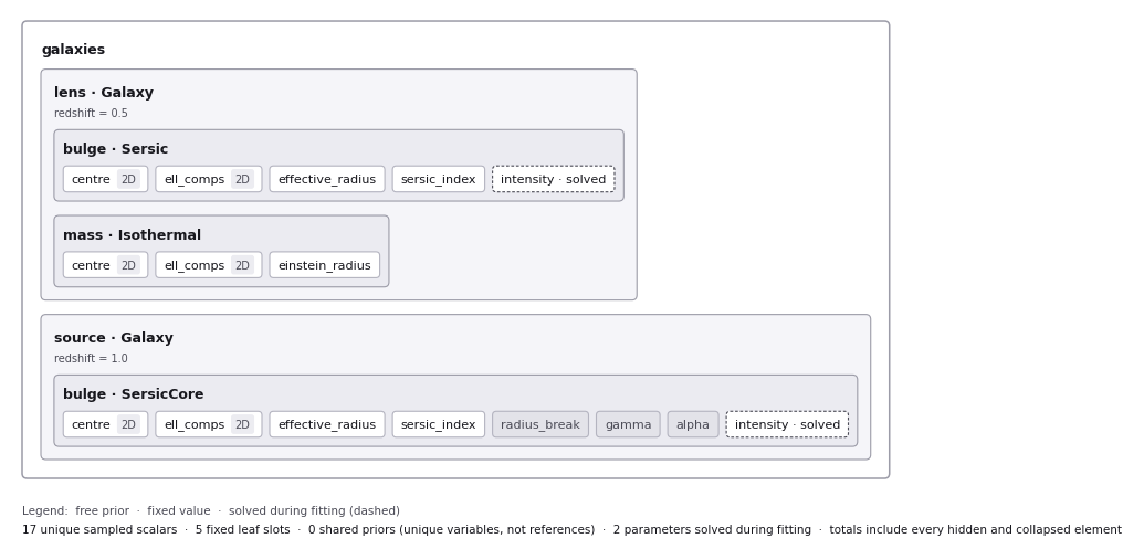
The simple lens model, drawn as nested component cards with one pill per parameter.

Every stage below prints model.info in the same way; from here on only the figure is shown.

More Complex Lens Models#

The API above can be easily extended to compose lens models where each galaxy has multiple light or mass profiles:

# Lens:

bulge = af.Model(al.lp_linear.Sersic)
disk = af.Model(al.lp_linear.Exponential)

mass = af.Model(al.mp.Isothermal)
shear = af.Model(al.mp.ExternalShear)

lens = af.Model(
    al.Galaxy,
    redshift=0.5,
    bulge=bulge,
    disk=disk,
    mass=mass,
    shear=shear,
)

# Source:

bulge = af.Model(al.lp_linear.SersicCore)
disk = af.Model(al.lp_linear.ExponentialCore)

source = af.Model(al.Galaxy, redshift=1.0, bulge=bulge, disk=disk)

# Overall Lens Model:

model = af.Collection(galaxies=af.Collection(lens=lens, source=source))

af.ModelPlotter(model).figure()

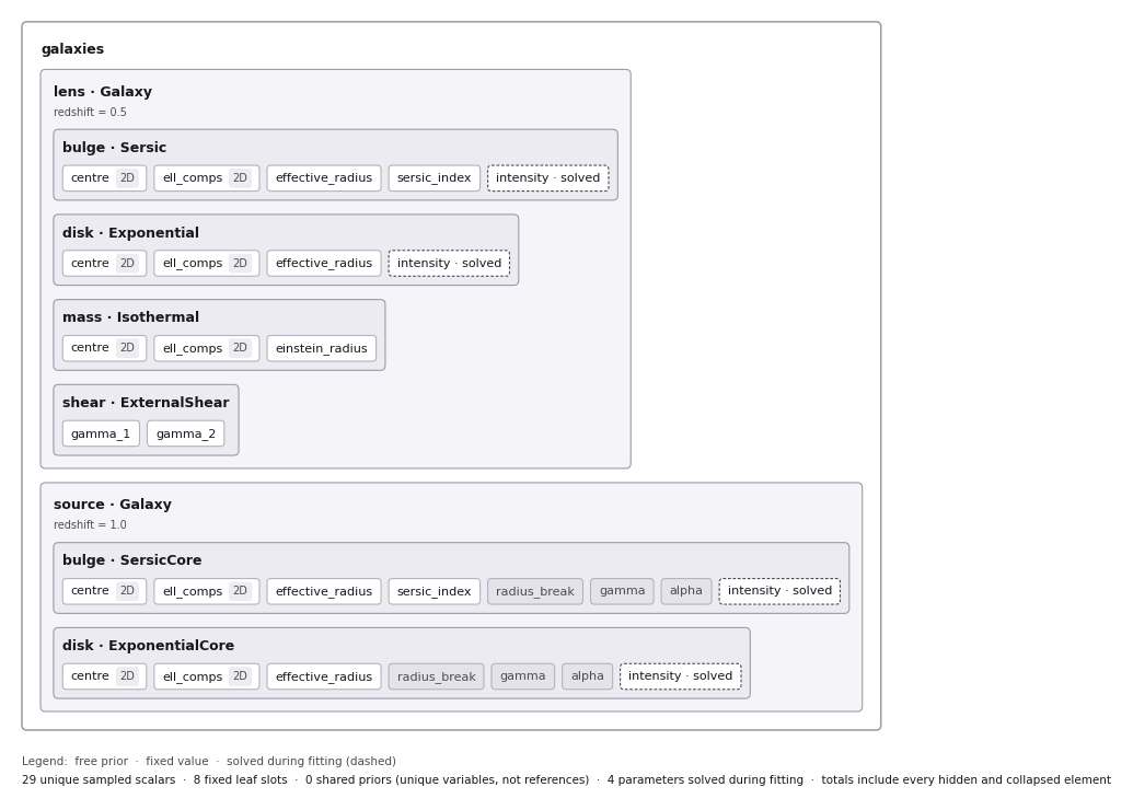
A lens model whose lens and source galaxies each have a bulge and a disk, with an external shear.

The use of the words bulge, disk, mass and shear above are arbitrary. They can be replaced with any name you like, e.g. bulge_0, bulge_1, mass_0, mass_1, and the model will still behave in the same way.

The API can also be extended to compose lens models where there are multiple galaxies:

bulge = af.Model(al.lp_linear.Sersic)
mass = af.Model(al.mp.Isothermal)

lens_0 = af.Model(
    al.Galaxy,
    redshift=0.5,
    bulge=bulge,
    mass=mass,
)

bulge = af.Model(al.lp_linear.Sersic)
mass = af.Model(al.mp.Isothermal)

lens_1 = af.Model(
    al.Galaxy,
    redshift=0.5,
    bulge=bulge,
    mass=mass,
)

# Source 0:

bulge = af.Model(al.lp_linear.SersicCore)

source_0 = af.Model(al.Galaxy, redshift=1.0, bulge=bulge)

# Source 1 :

bulge = af.Model(al.lp_linear.SersicCore)

source_1 = af.Model(al.Galaxy, redshift=1.0, bulge=bulge)

# Overall Lens Model:

model = af.Collection(
    galaxies=af.Collection(
        lens_0=lens_0,
        lens_1=lens_1,
        source_0=source_0,
        source_1=source_1
    )
)

af.ModelPlotter(model).figure()

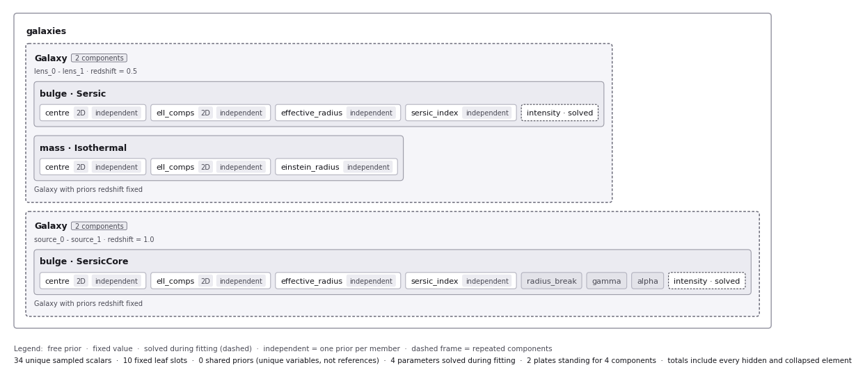
A lens model with two lens galaxies and two source galaxies.

The two lens galaxies are identical in structure, and so are the two source galaxies, but their parameters are independent: two separate priors with the same configuration, which is not the same thing as one shared prior.

The above lens model consists of only two planes (an image-plane and source-plane), but has four galaxies in total. This is because the lens galaxies have the same redshift and the source galaxies have the same redshift.

If we gave one of the lens galaxies a different redshift, it would be included in a third plane, and the model would perform multi-plane ray tracing when the model-fit is performed.

Concise API#

If a light or mass profile is passed directly to the af.Model of a galaxy, it is automatically assigned to be a af.Model component of the galaxy.

This means we can write the model above comprising multiple light and mass profiles more concisely as follows (also removing the comments reading Lens / Source / Overall Lens Model to make the code more readable):

lens = af.Model(
    al.Galaxy,
    redshift=0.5,
    bulge=al.lp_linear.Sersic,
    disk=al.lp_linear.Sersic,
    mass=al.mp.Isothermal,
    shear=al.mp.ExternalShear,
)

source = af.Model(
    al.Galaxy,
    redshift=1.0,
    bulge=al.lp_linear.SersicCore,
    disk=al.lp_linear.ExponentialCore,
)

model = af.Collection(galaxies=af.Collection(lens=lens, source=source))

af.ModelPlotter(model).figure()

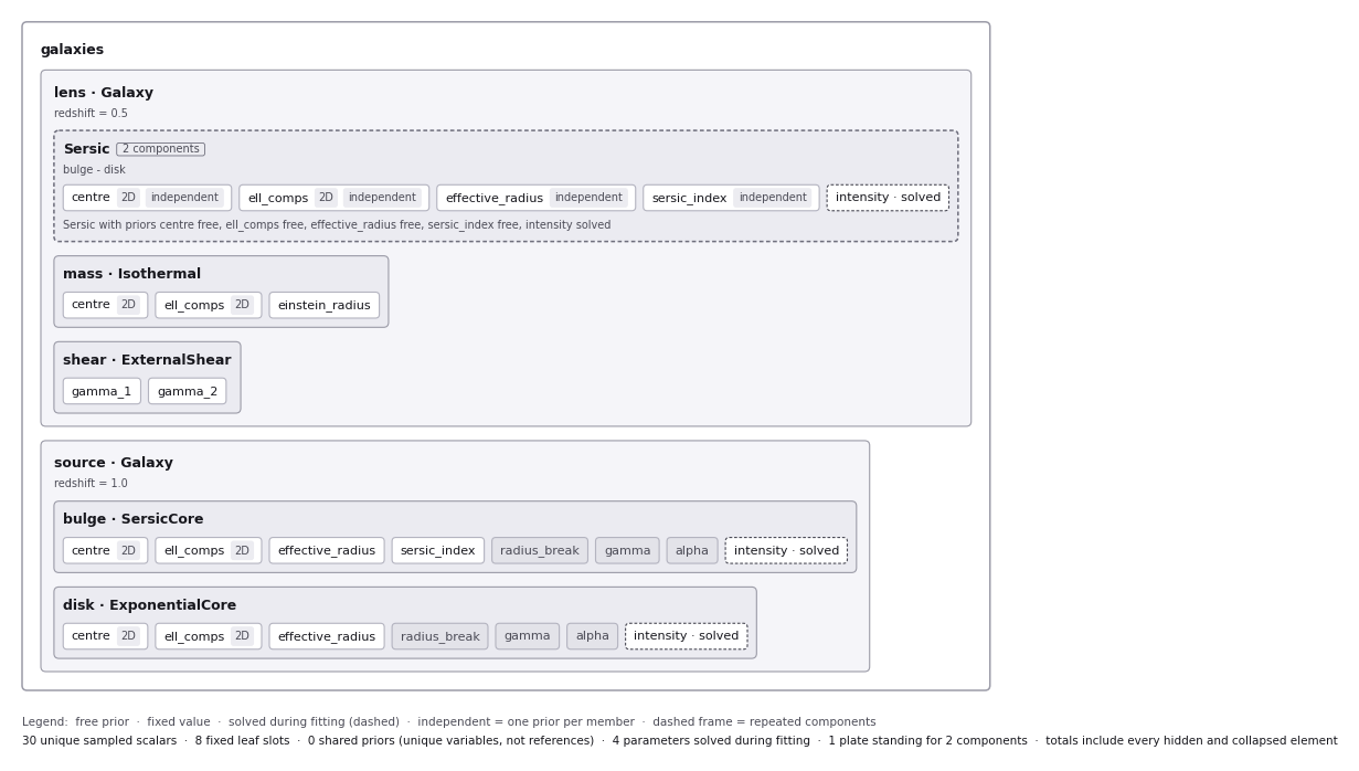
The same lens and source model composed with the concise API.

The concise API is a shorthand for writing a model, not a different model. Note that this stage gives the lens galaxy a Sersic bulge and a Sersic disk, and each of the two has its own priors rather than sharing one.

Prior Customization#

We can customize the priors of the lens model component individual parameters, using the following three types of priors:

UniformPrior: The values of a parameter are randomly drawn between a lower_limit and upper_limit. For example, the effective radius of elliptical Sersic profiles typically assumes a uniform prior between 0.0” and 30.0”.

LogUniformPrior: Like a UniformPrior this randomly draws values between a lower_limit and upper_limit, but the values are drawn from a distribution with base 10. This is used for the intensity of a light profile, as the luminosity of galaxies follows a log10 distribution.

GaussianPrior: The values of a parameter are randomly drawn from a Gaussian distribution with a mean and width sigma. For example, the $y$ and $x$ centre values in a light profile typically assume a mean of 0.0” and a sigma of 0.3”, indicating that we expect the profile centre to be located near the centre of the image.

# Lens:

bulge = af.Model(al.lp_linear.Sersic)
bulge.sersic_index = af.TruncatedGaussianPrior(
    mean=4.0, sigma=1.0, lower_limit=1.0, upper_limit=8.0
)

mass = af.Model(al.mp.Isothermal)
mass.centre.centre_0 = af.TruncatedGaussianPrior(
    mean=0.0, sigma=0.1, lower_limit=-0.5, upper_limit=0.5
)
mass.centre.centre_1 = af.TruncatedGaussianPrior(
    mean=0.0, sigma=0.1, lower_limit=-0.5, upper_limit=0.5
)
mass.einstein_radius = af.UniformPrior(lower_limit=0.0, upper_limit=8.0)

lens = af.Model(
    al.Galaxy,
    redshift=0.5,
    bulge=bulge,
    mass=mass,
)

# Source

bulge = af.Model(al.lp_linear.SersicCore)

source = af.Model(al.Galaxy, redshift=1.0, bulge=bulge)
source.effective_radius = af.TruncatedGaussianPrior(
    mean=0.1, sigma=0.05, lower_limit=0.0, upper_limit=1.0
)

# Overall Lens Model:

model = af.Collection(galaxies=af.Collection(lens=lens, source=source))

af.ModelPlotter(model).figure()

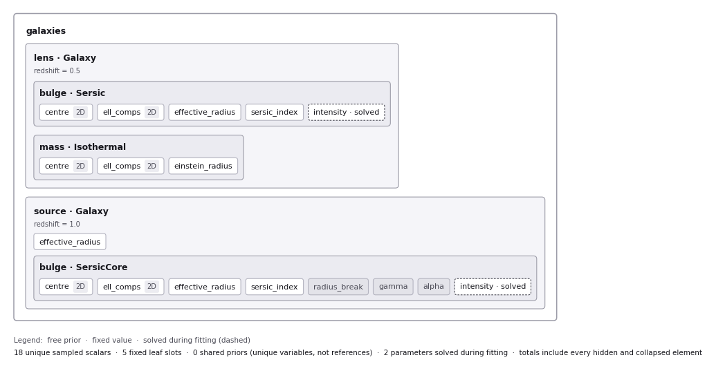
A lens model whose sersic index, mass centre and einstein radius priors have been customized.

Customizing a prior does not change a parameter’s state — a parameter with a customized prior is still sampled. Print model.info, or call af.ModelPlotter(model).figure(detail="priors"), to read the prior on each parameter.

One thing in the code above is easy to misread: the last line sets effective_radius on the source galaxy, not on the source galaxy’s bulge. A Galaxy accepts any attribute, so this adds a new free effective_radius parameter to the source galaxy itself rather than overriding the bulge’s own prior. Writing source.bulge.effective_radius = ... is what customizes the bulge.

Model Customization#

We can customize the lens model parameters in a number of different ways, as shown below:

# Lens:

bulge = af.Model(al.lp_linear.Sersic)
disk = af.Model(al.lp_linear.Exponential)

# Parameter Pairing: Pair the centre of the bulge and disk together, reducing
# the complexity of non-linear parameter space by N = 2

bulge.centre = disk.centre

# Parameter Fixing: Fix the sersic_index of the bulge to a value of 4, reducing
# the complexity of non-linear parameter space by N = 1

bulge.sersic_index = 4.0

mass = af.Model(al.mp.Isothermal)

# Parameter Offsets: Make the mass model centre parameters the same value as
# the bulge / disk but with an offset.

mass.centre.centre_0 = bulge.centre.centre_0 + 0.1
mass.centre.centre_1 = bulge.centre.centre_1 + 0.1

shear = af.Model(al.mp.ExternalShear)

lens = af.Model(
    al.Galaxy,
    redshift=0.5,
    bulge=bulge,
    disk=disk,
    mass=mass,
    shear=shear,
)

# Source:

bulge = af.Model(al.lp_linear.SersicCore)
disk = af.Model(al.lp_linear.ExponentialCore)

source = af.Model(al.Galaxy, redshift=1.0, bulge=bulge, disk=disk)

# Overall Lens Model:

model = af.Collection(galaxies=af.Collection(lens=lens, source=source))

# Assert that the effective radius of the bulge is larger than that of the disk.
# (Assertions can only be added at the end of model composition, after all components
# have been brought together in a `Collection`.
model.add_assertion(model.galaxies.lens.bulge.effective_radius > model.galaxies.lens.disk.effective_radius)

# Assert that the Einstein Radius is below 3.0":
model.add_assertion(model.galaxies.lens.mass.einstein_radius < 3.0)

af.ModelPlotter(model).figure()

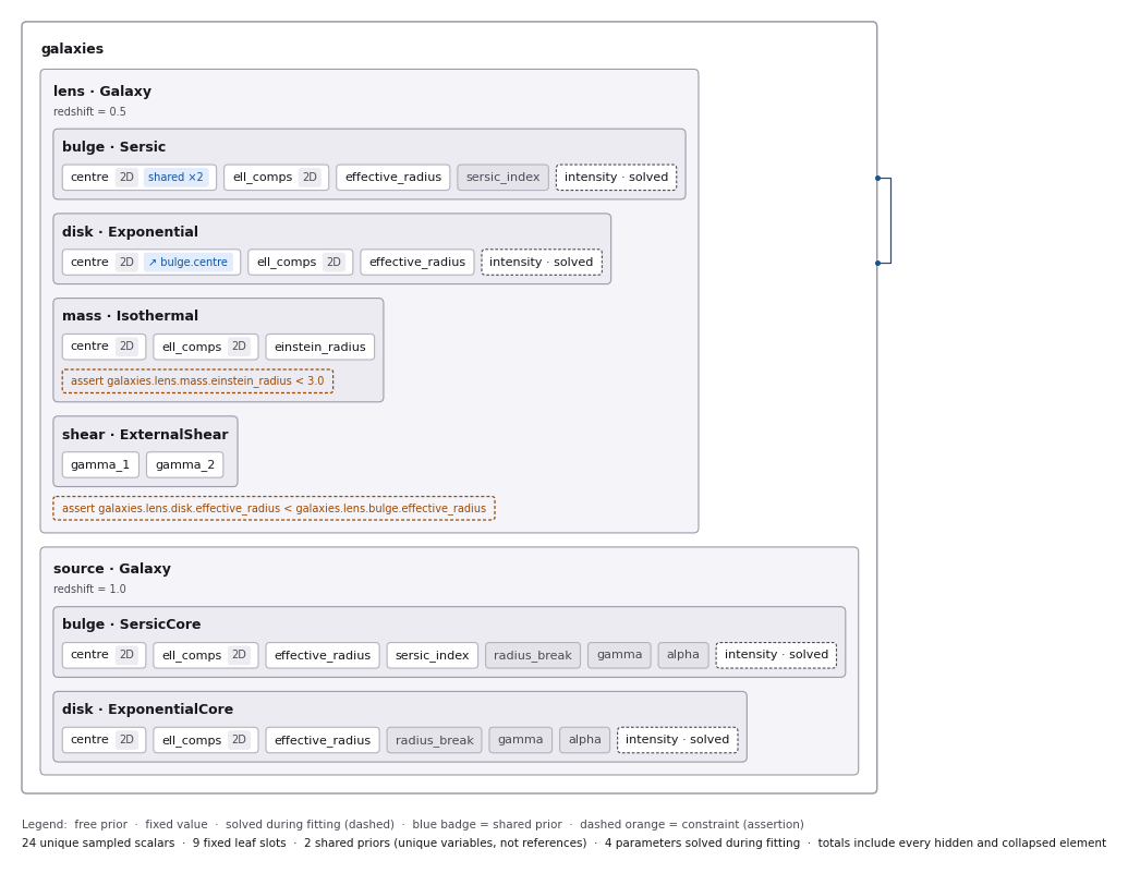
A customized lens model showing a paired centre, a fixed sersic index, offset relations and two assertions.

The disk reuses the bulge’s centre rather than having one of its own, the sersic_index is fixed, and the model carries two assertions relating its parameters.

The two offset centre components of the mass profile are a relation: they are defined by an expression rather than sampled. A relation on one component of a tuple parameter such as centre is not yet annotated on the model figure, so model.info is the place to read it.

Redshift Free#

The redshift of a galaxy can be treated as a free parameter in the model-fit by using the following API:

redshift = af.Model(al.Redshift)
redshift.redshift = af.UniformPrior(lower_limit=0.0, upper_limit=2.0)

lens = af.Model(
    al.Galaxy,
    redshift=redshift,
    mass=al.mp.Isothermal
)

source = af.Model(al.Galaxy, redshift=1.0, bulge=al.lp_linear.SersicCore)

model = af.Collection(galaxies=af.Collection(lens=lens, source=source))

af.ModelPlotter(model).figure()

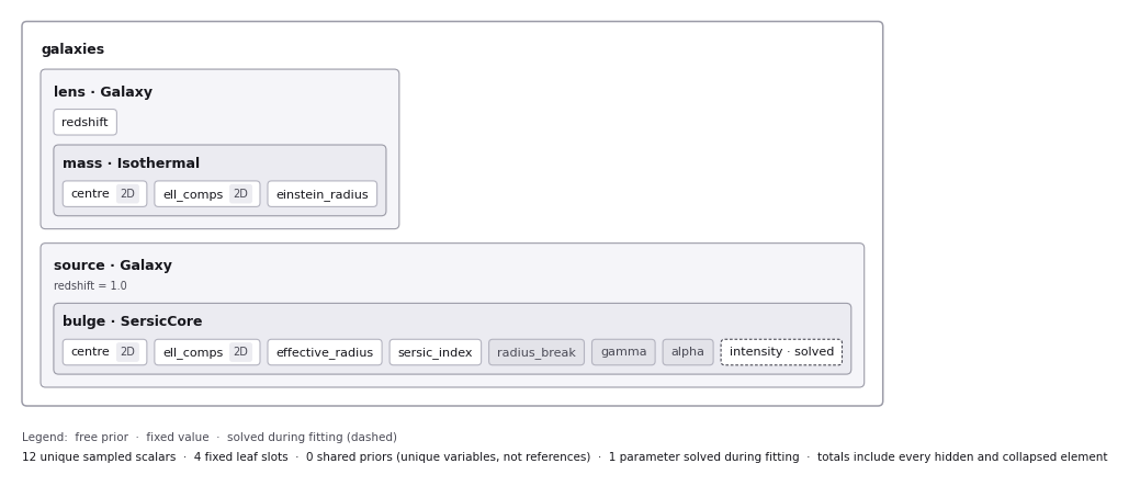
A lens model whose lens galaxy redshift is a free parameter, drawn as an ordinary pill on the galaxy card.

A free redshift is an ordinary sampled parameter of the galaxy. A fixed redshift is not a parameter of the model at all, and the source galaxy above shows this.

The model-fit will automatically enable multi-plane ray tracing and alter the ordering of the planes depending on the redshifts of the galaxies.

NOTE: For strong lenses with just two planes (an image-plane and source-plane) the redshifts of the galaxies do not impact the model-fit. You should therefore never make the redshifts free if you are only modeling a two-plane lens system. This is because lensing calculations can be defined in arc-second coordinates, which do not change as a function of redshift.

Redshifts should be made free when modeling three or more planes, as the multi-plane ray-tracing calculations have an obvious dependence on the redshifts of the galaxies which could be inferred by the model-fit.

Solved and Unconfigured Parameters#

Some parameters of a lens model are neither sampled by the non-linear search nor fixed by the user: they are solved for during the fit, at every likelihood evaluation. The model below contains all three of them:

# Lens: a linear light profile, whose `intensity` is solved for by the inversion.

lens = af.Model(
    al.Galaxy,
    redshift=0.5,
    bulge=af.Model(al.lp_linear.Sersic),
    mass=af.Model(al.mp.Isothermal),
)

# Source: a pixelization, whose source `reconstruction` is solved for by the inversion.

pixelization = af.Model(
    al.Pixelization,
    mesh=af.Model(al.mesh.Delaunay, pixels=500, zeroed_pixels=0),
    regularization=af.Model(al.reg.ConstantSplit),
)

source = af.Model(al.Galaxy, redshift=1.0, pixelization=pixelization)

# Point source: a `PointSolved`, whose `centre` is solved for analytically.

point_source = af.Model(al.Galaxy, redshift=1.0, point=af.Model(al.ps.PointSolved))

model = af.Collection(
    galaxies=af.Collection(lens=lens, source=source, point_source=point_source)
)

af.ModelPlotter(model).figure()

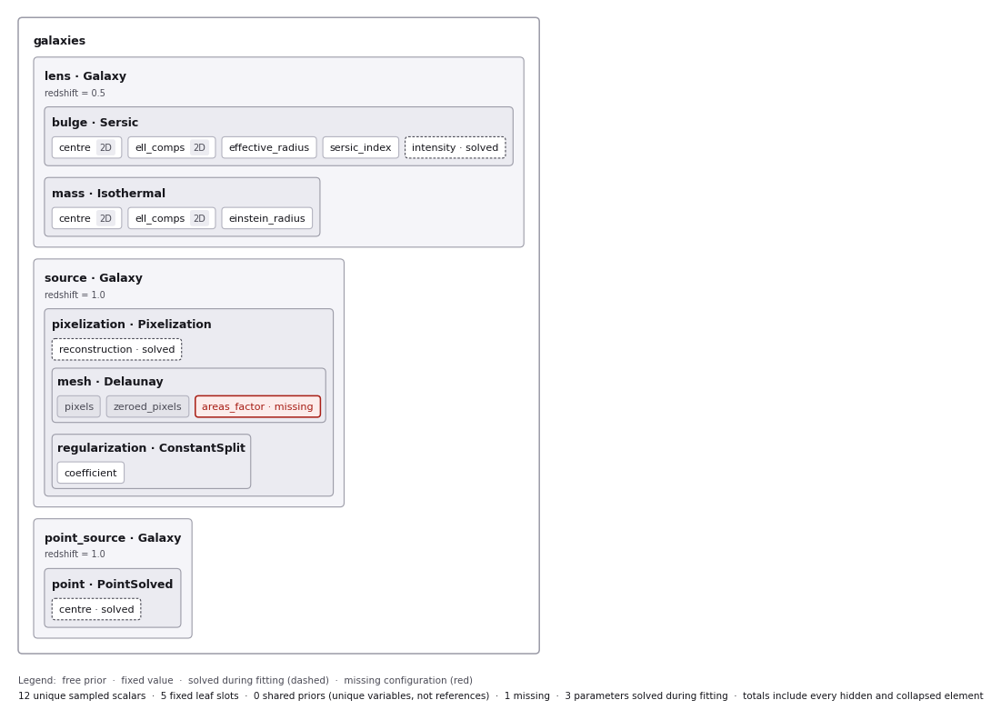
A lens model showing the three solved parameters and one missing configuration value.

Three parameters of this model are solved for during the fit:

the intensity of every linear light profile (al.lp_linear.*, and every member of an al.lp_basis.Basis built from them), which the inversion solves for by linear algebra rather than the search sampling it. A Basis has no solved amplitude of its own: the solved intensities belong to its member profiles, one per member.
the reconstruction of an al.Pixelization, which is the solved surface brightness of every source pixel. The only sampled parameters of a pixelization are its regularization coefficients.
the centre of an al.ps.PointSolved, which is solved for analytically by the *Solved point-source fit classes. al.ps.Point, by contrast, samples its centre as an ordinary free parameter.

These three have no counterpart in model.info at all, because they are not sampled parameters of the model.

A different thing again is areas_factor, a parameter of the Delaunay mesh for which no prior is configured, so the model cannot be fitted until one is supplied (via config/priors or by setting it in the script). It is unset configuration — not solved, and not absent from the model.

PyAutoLens’ own default configuration ships no prior for areas_factor. The autolens_workspace supplies one in config/priors/mesh/delaunay.yaml, as a constant 0.5, so the same code run from the workspace has an ordinary fixed parameter instead: unset configuration is what you see when your own configuration has a gap.

Available Model Components#

The light profiles, mass profiles and other components that can be used for lens modeling are given at the following API documentation pages:

https://pyautolens.readthedocs.io/en/latest/api/light.html

https://pyautolens.readthedocs.io/en/latest/api/mass.html

https://pyautolens.readthedocs.io/en/latest/api/pixelization.html

JSon Outputs#

After a model is composed, it can easily be output to a .json file on hard-disk in a readable structure:

import os
import json

model_path = path.join("path", "to", "model", "json")

os.makedirs(model_path, exist_ok=True)

model_file = path.join(model_path, "model.json")

with open(model_file, "w+") as f:
    json.dump(model.dict(), f, indent=4)

We can load the model from its .json file.

model = af.Model.from_json(file=model_file)

This means in PyAutoLens one can write a model in a script, save it to hard disk and load it elsewhere, as well as manually customize it in the .json file directory.

This is used for composing complex models of group scale lenses.

Multi Galaxy, Group and Cluster Models#

Above galaxy scale, models are composed for three regimes (see the New User Guide’s “What Scale System?” ladder — all groups and clusters are multi-galaxy systems, but not vice versa):

Multi-galaxy lenses (2+ co-dominant deflectors, no host halo): one free light + mass model per deflector, composed in a loop with untruncated isothermals (no host halo means no tidal truncation):

lens_dict = {}

for i, centre in enumerate(main_lens_centres):
    mass = af.Model(al.mp.Isothermal)
    mass.centre = (centre[0], centre[1])

    lens_dict[f"lens_{i}"] = af.Model(al.Galaxy, redshift=0.5, mass=mass)

model = af.Collection(galaxies=af.Collection(**lens_dict, source=source))

Group-scale lenses add two things as explicit modelling choices: an optional dark-matter group halo, and faint members whose masses are tied to their luminosities through a shared scaling relation, so N galaxies cost one free parameter (composed via prior arithmetic on a shared prior):

einstein_radius_ref = af.UniformPrior(lower_limit=0.0, upper_limit=1.0)

for i, (centre, luminosity) in enumerate(zip(centres, luminosities)):
    mass = af.Model(al.mp.IsothermalSph)
    mass.centre = (centre[0], centre[1])
    mass.einstein_radius = einstein_radius_ref * (luminosity / reference_luminosity) ** 0.5

Cluster-scale lenses keep the group mass framework (halo + tidally truncated dPIE members on scaling relations) but change the source strategy: many point-source multiple-image position datasets, each at its own redshift, fitted via AnalysisPoint.

The full group-scale composition — one main lens galaxy with an external shear, a SersicCore source and one extra galaxy per detected group member, each with a SersicSph light profile and a dPIEMassSph mass profile whose centre is fixed to its measured position — is the script autolens_workspace/scripts/group/modeling.py. Drawn as a figure, with eight extra galaxies, it looks like this:

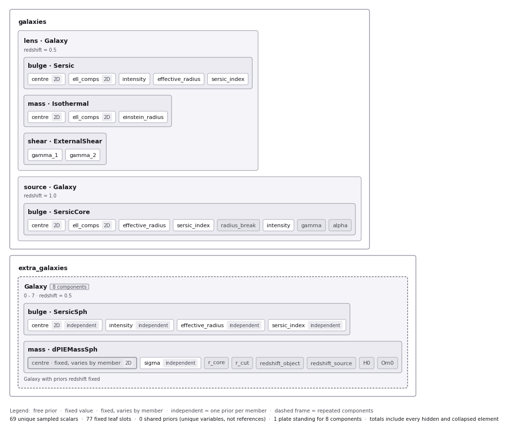
A group-scale lens model, whose eight extra galaxies collapse into a single plate of eight components.

The eight extra galaxies are identical in structure, but each has its own fixed centre rather than one centre common to all, and each has its own sigma prior, because eight separate priors with the same configuration is not the same thing as one shared prior.

The following example notebooks show each regime’s full model composition:

https://github.com/PyAutoLabs/autolens_workspace/blob/main/notebooks/multi_galaxy/modeling.ipynb https://github.com/PyAutoLabs/autolens_workspace/blob/main/notebooks/group/modeling.ipynb https://github.com/PyAutoLabs/autolens_workspace/blob/main/notebooks/group/start_here.ipynb https://github.com/PyAutoLabs/autolens_workspace/blob/main/notebooks/group/features/group_halo/modeling.ipynb https://github.com/PyAutoLabs/autolens_workspace/blob/main/notebooks/cluster/start_here.ipynb

Many Profile Models (Advanced)#

Features such as the Multi Gaussian Expansion (MGE) and shapelets compose models consisting of 50 - 500+ light profiles.

An MGE lens light model of 2 x 30 linear Gaussians, fitted alongside a pixelized source, draws like this:

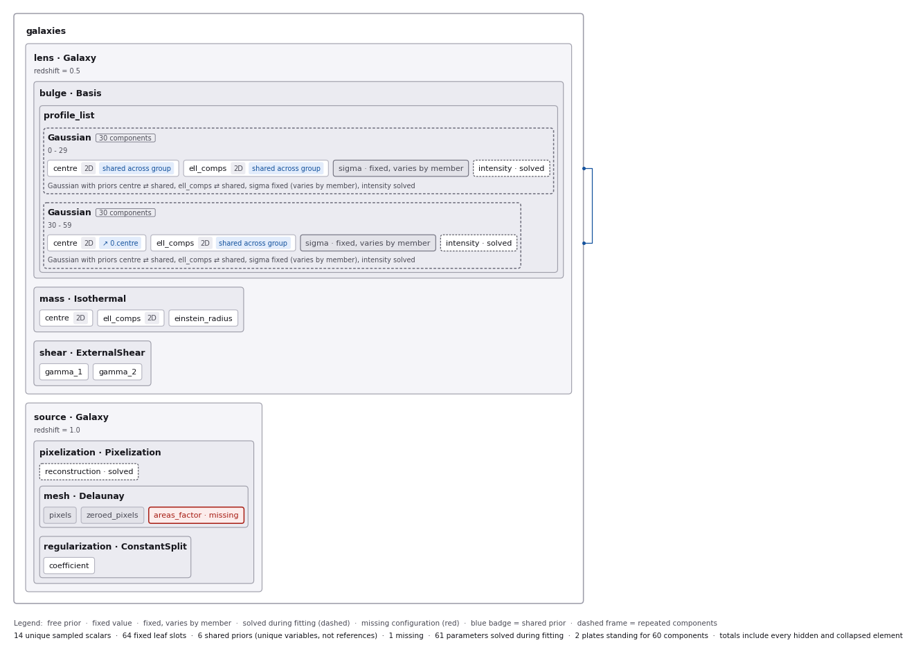
The 60 Gaussians are split across two bases, because each basis holds its own ell_comps pair while all 60 share one centre. Every member’s intensity is solved for by the inversion, as is the source’s reconstruction, and the mesh’s areas_factor has no prior configured.

The following example notebooks show how to compose and fit these models:

https://github.com/PyAutoLabs/autolens_workspace/blob/main/notebooks/imaging/features/multi_gaussian_expansion/modeling.ipynb https://github.com/PyAutoLabs/autolens_workspace/blob/main/notebooks/imaging/features/advanced/shapelets/modeling.ipynb

Model Linking (Advanced)#

When performing non-linear search chaining, the inferred model of one phase can be linked to the model.

For a model with a separate external field, carry the mass and field together:

mass, field = al.util.chaining.mass_and_fields_from(
    mass=af.Model(al.mp.PowerLaw),
    mass_result=result_1.model.galaxies.lens.mass,
    fields_result=result_1.model.fields,
)
model_2 = af.Collection(
    galaxies=af.Collection(lens=af.Model(al.Galaxy, redshift=0.5, mass=mass), source=source),
    fields=field,
)

result_1.model.fields passes posterior priors into the next stage; use result_1.instance.fields to fix the field to the previous fit’s values.

The following example notebooks show how to compose and fit these models:

https://github.com/PyAutoLabs/autolens_workspace/blob/main/notebooks/guides/modeling/chaining.ipynb

Across Datasets (Advanced)#

When fitting multiple datasets, model can be composed where the same model component are used across the datasets but certain parameters are free to vary across the datasets.

The following example notebooks show how to compose and fit these models:

https://github.com/PyAutoLabs/autolens_workspace/blob/main/notebooks/multi_dataset/start_here.ipynb

Relations (Advanced)#

We can compose models where the free parameter(s) vary according to a user-specified function (e.g. y = mx +c -> intensity = (m * wavelength) + c across the datasets.

The following example notebooks show how to compose and fit these models:

https://github.com/PyAutoLabs/autolens_workspace/blob/main/notebooks/multi_dataset/features/wavelength_dependence/modeling.ipynb

PyAutoFit API#

PyAutoFit is a general model composition library which offers even more ways to compose lens models not detailed in this cookbook.

The PyAutoFit model composition cookbooks detail this API in more detail:

https://pyautofit.readthedocs.io/en/latest/cookbooks/model.html https://pyautofit.readthedocs.io/en/latest/cookbooks/multi_level_model.html

Wrap Up#

This cookbook shows how to compose simple lens models using the af.Model() and af.Collection() objects.