Group-Scale Lenses

The strong lenses we’ve discussed so far have just a single lens galaxy responsible for the lensing, with a single source galaxy observed.

A strong lensing group is a system which has a distinct ‘primary’ lens galaxy and a handful of lower mass galaxies nearby. They typically contain just one or two lensed sources whose arcs are extended and visible. Their Einstein Radii range between typical values of 5.0” -> 10.0” and with care, it is feasible to fit the source’s extended emission in the imaging or interferometer data.

Strong lensing clusters, which contain many hundreds of lens and source galaxies, cannot be modeled with PyAutoLens. However, we are actively developing this functionality.

Dataset

Lets begin by looking at a simulated group-scale strong lens which clearly has a distinct primary lens galaxy, but additional galaxies can be seen in and around the Einstein ring.

These galaxies are faint and small in number, but their lensing effects on the source are significant enough that we must ultimately include them in the lens model.

import autolens as al
import autolens.plot as aplt

dataset_name = "lens_x3__source_x1"
dataset_path = path.join("dataset", "group", dataset_name)

dataset = al.Imaging.from_fits(
    data_path=path.join(dataset_path, "data.fits"),
    noise_map_path=path.join(dataset_path, "noise_map.fits"),
    psf_path=path.join(dataset_path, "psf.fits"),
    pixel_scales=0.1,
)

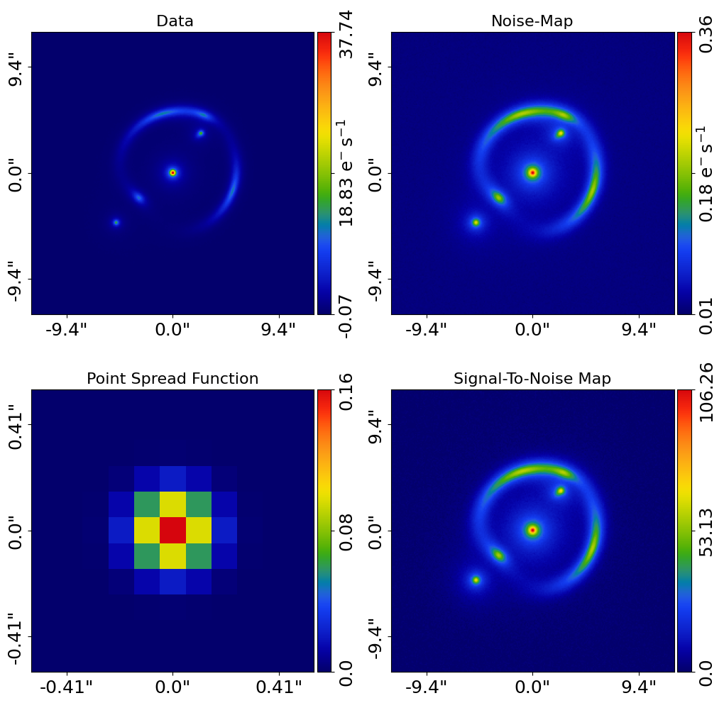
dataset_plotter = aplt.ImagingPlotter(dataset=dataset)
dataset_plotter.subplot_dataset()

Here is what the group-scale lens looks like.

The Source’s ring is much larger than other examples (> 5.0”) and there are clearly additional galaxies in and around the main lens galaxy.

Point Source

Modeling group scale lenses is challenging, because each individual galaxy must be included in the overall lens model. For this simple overview, we will therefore model the system as a point source, which reduces the complexity of the model and reduces the computational run-time of the model-fit.

Lets the lens’s point-source data, where the brightest pixels of the source are used as the locations of its centre.

point_dict = al.PointDict.from_json(
    file_path=path.join(dataset_path, "point_dict.json")
)

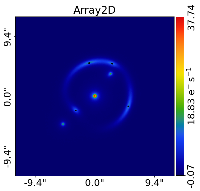
We plot its positions over the observed image, using the Visuals2D object:

visuals = aplt.Visuals2D(positions=point_dict.positions_list)

array_plotter = aplt.Array2DPlotter(array=dataset.data, visuals_2d=visuals)
array_plotter.figure_2d()

Here is what it looks like:

Model via JSON

We now compose the lens model. For groups there could be many lens and source galaxies in the model.

Whereas previous examples explicitly wrote the model out via Python code, for group modeling we opt to write it in .json files which are loaded in this script.

The code below loads a model from a .json file created by the script group/models/lens_x3__source_x1.py. This model includes all three lens galaxies where the priors on the centres have been paired to the brightest pixels in the observed image, alongside a source galaxy which is modeled as a point source.

model_path = path.join("dataset", "group", "lens_x3__source_x1")

lenses_file = path.join(model_path, "lenses.json")
lenses = af.Collection.from_json(file=lenses_file)

sources_file = path.join(model_path, "sources.json")
sources = af.Collection.from_json(file=sources_file)

galaxies = lenses + sources

model = af.Collection(galaxies=galaxies)

This .json file contains all the information on this particular lens’s model, including priors which adjust their centre to the centre of light of each lens galaxy. The script used to make the model can be viewed at the following link.

The model can be displayed via its info property:

print(model.info)

Here is how the model appears when printed:

Total Free Parameters = 13

model                             Collection (N=13)
    galaxies                      Collection (N=13)
        lens_0                    Galaxy (N=5)
            mass                  IsothermalSph (N=3)
            shear                 ExternalShear (N=2)
        lens_1                    Galaxy (N=3)
            mass                  IsothermalSph (N=3)
        lens_2                    Galaxy (N=3)
            mass                  IsothermalSph (N=3)
        source_0                  Galaxy (N=2)
            point_0               PointSourceChi (N=2)

galaxies
    lens_0
        redshift                  0.5
        mass
            centre
                centre_0          GaussianPrior [4], mean = 0.0, sigma = 0.5
                centre_1          GaussianPrior [5], mean = 0.0, sigma = 0.5
            einstein_radius       UniformPrior [6], lower_limit = 0.0, upper_limit = 8.0
        shear
            gamma_1               UniformPrior [9], lower_limit = -0.2, upper_limit = 0.2
            gamma_2               UniformPrior [10], lower_limit = -0.2, upper_limit = 0.2
    lens_1
        redshift                  0.5
        mass
            centre
                centre_0          GaussianPrior [14], mean = 3.5, sigma = 0.5
                centre_1          GaussianPrior [15], mean = 2.5, sigma = 0.5
            einstein_radius       UniformPrior [16], lower_limit = 0.0, upper_limit = 8.0
    lens_2
        redshift                  0.5
        mass
            centre
                centre_0          GaussianPrior [20], mean = -4.4, sigma = 0.5
                centre_1          GaussianPrior [21], mean = -5.0, sigma = 0.5
            einstein_radius       UniformPrior [22], lower_limit = 0.0, upper_limit = 8.0
    source_0
        redshift                  1.0
        point_0
            centre
                centre_0          GaussianPrior [25], mean = 0.0, sigma = 3.0
                centre_1          GaussianPrior [26], mean = 0.0, sigma = 3.0

The source does not use the Point class discussed in the previous overview example, but instead uses a PointSourceChi object.

This object changes the behaviour of how the positions in the point dataset are fitted. For a normal Point object, the positions are fitted in the image-plane, by mapping the source-plane back to the image-plane via the lens model and iteratively searching for the best-fit solution.

The PointSourceChi object instead fits the positions directly in the source-plane, by mapping the image-plane positions to the source just one. This is a much faster way to fit the positions,and for group scale lenses it typically sufficient to infer an accurate lens model.

Lens Modeling

We are now able to model this dataset as a point source, using the exact same tools we used in the point source overview.

search = af.Nautilus(name="overview_groups")

analysis = al.AnalysisPoint(point_dict=point_dict, solver=None)

result = search.fit(model=model, analysis=analysis)

Result

The result contains information on every galaxy in our lens model:

print(result.max_log_likelihood_instance.galaxies.lens_0.mass)
print(result.max_log_likelihood_instance.galaxies.lens_1.mass)
print(result.max_log_likelihood_instance.galaxies.lens_2.mass)

Extended Source Fitting

For group-scale lenses like this one, with a modest number of lens and source galaxies, PyAutoLens has all the tools you need to perform extended surface-brightness fitting to the source’s extended emission, including the use of a pixelized source reconstruction.

This will extract a lot more information from the data than the point-source model and the source reconstruction means that you can study the properties of the highly magnified source galaxy. Here is what the fit looks like:

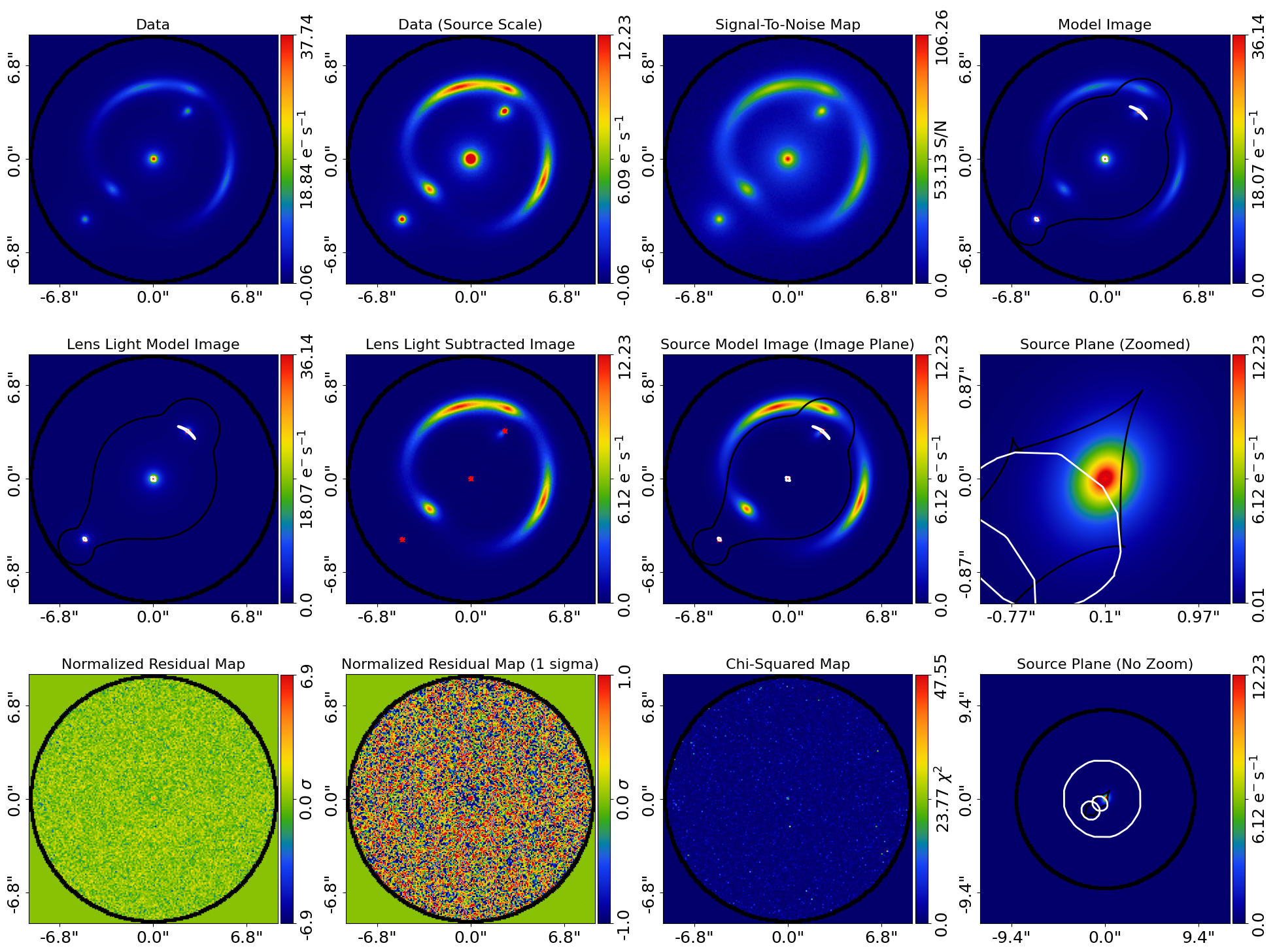
For group-scale lenses like this one, with a modest number of lens and source galaxies it is feasible to perform extended surface-brightness fitting to the source’s extended emission. This includes using a pixelized source reconstruction.

This will extract a lot more information from the data than the point-source model and the source reconstruction means that you can study the properties of the highly magnified source galaxy.

This type of modeling uses a lot of PyAutoLens’s advanced model-fitting features which are described in chapters 3 and 4 of the HowToLens tutorials. An example performing this analysis to the lens above can be found at this link.

Wrap-Up

The group package of the autolens_workspace contains numerous example scripts for performing group-sale modeling and simulating group-scale strong lens datasets.