Lens Modeling#
Lens modeling is the process of taking data of a strong lens (e.g. imaging data from the Hubble Space Telescope or interferometer data from ALMA) and fitting it with a lens model, to determine the light and mass distributions of the lens and source galaxies that best represent the observed strong lens.
Dataset#
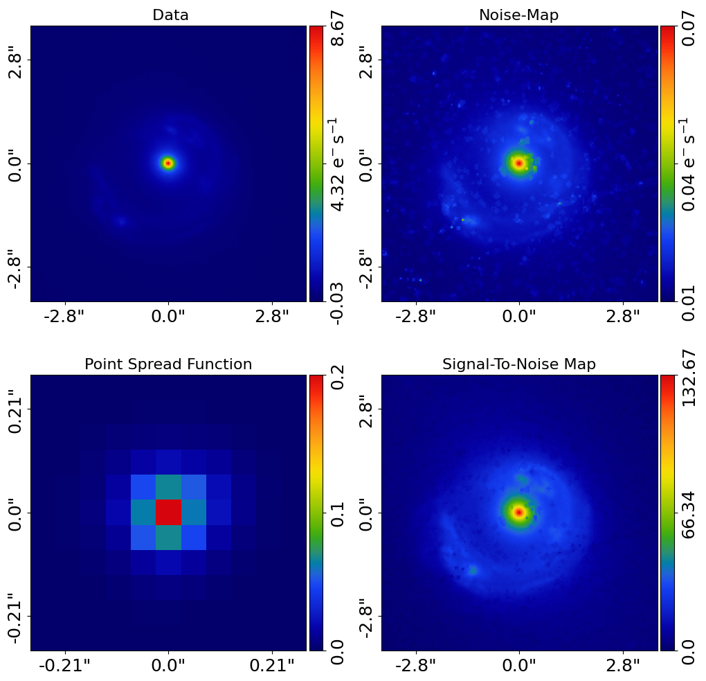
In this example, we model Hubble Space Telescope imaging of a real strong lens system, with our goal to infer the lens and source galaxy light and mass models that fit the data well!
import autolens as al
import autolens.plot as aplt

dataset_path = path.join("dataset", "slacs", "slacs1430+4105")

dataset = al.Imaging.from_fits(
    data_path=path.join(dataset_path, "data.fits"),
    psf_path=path.join(dataset_path, "psf.fits"),
    noise_map_path=path.join(dataset_path, "noise_map.fits"),
    pixel_scales=0.05,
)

dataset_plotter = aplt.ImagingPlotter(dataset=dataset)
dataset_plotter.subplot_dataset()
Here is what the dataset looks like:
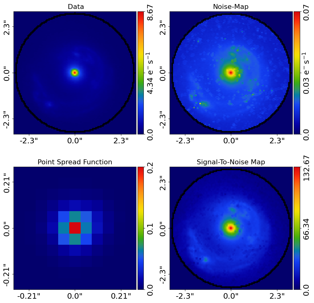
We next mask the dataset, to remove the exterior regions of the image that do not contain emission from the lens or source galaxy.
mask = al.Mask2D.circular(
    shape_native=dataset.shape_native, pixel_scales=dataset.pixel_scales, radius=3.0
)

dataset = dataset.apply_mask(mask=mask)

dataset_plotter = aplt.ImagingPlotter(dataset=dataset)
dataset_plotter.subplot_dataset()
Note how when we plot the Imaging below, the figure now zooms into the masked region.
PyAutoFit#
Lens modeling uses the probabilistic programming language PyAutoFit, an open-source Python framework that allows complex model fitting techniques to be straightforwardly integrated into scientific modeling software. Check it out if you are interested in developing your own software to perform advanced model-fitting!
We import PyAutoFit separately to PyAutoLens
import autofit as af
Model Composition#
We compose the lens model that we fit to the data using af.Model objects.
These behave analogously to Galaxy objects but their LightProfile and MassProfile parameters are not specified, they are instead determined by a fitting procedure.
We will fit our strong lens data with two galaxies:
A lens galaxy with an Isothermal mass profile representing its mass, whose centre is fixed to (0.0”, 0.0”).
A source galaxy with an Exponential light profile representing a disk.
The redshifts of the lens (z=0.155) and source(z=0.517) are fixed.
# Lens:

mass = af.Model(al.mp.Isothermal)
mass.centre = (0.0, 0.0)

# Source:

disk = af.Model(al.lp.Exponential)

source = af.Model(al.Galaxy, redshift=0.517, disk=disk)
The info attribute of each Model component shows the model in a readable format.
print(lens.info)
This gives the following output:
Total Free Parameters = 8

model                                       Galaxy (N=8)
    bulge                                   Sersic (N=5)
    mass                                    Isothermal (N=3)

redshift                                    0.285
bulge
    centre                                  (0.0, 0.0)
    ell_comps
        ell_comps_0                         GaussianPrior [3], mean = 0.0, sigma = 0.3
        ell_comps_1                         GaussianPrior [4], mean = 0.0, sigma = 0.3
    intensity                               LogUniformPrior [5], lower_limit = 1e-06, upper_limit = 1000000.0
    effective_radius                        UniformPrior [6], lower_limit = 0.0, upper_limit = 30.0
    sersic_index                            UniformPrior [7], lower_limit = 0.8, upper_limit = 5.0
mass
    centre                                  (0.0, 0.0)
    ell_comps
        ell_comps_0                         GaussianPrior [10], mean = 0.0, sigma = 0.3
        ell_comps_1                         GaussianPrior [11], mean = 0.0, sigma = 0.3
    einstein_radius                         UniformPrior [12], lower_limit = 0.0, upper_limit = 8.0

Total Free Parameters = 6

model                                       Galaxy (N=6)
    disk                                    Exponential (N=6)

redshift                                    0.575
disk
    centre
        centre_0                            GaussianPrior [13], mean = 0.0, sigma = 0.3
        centre_1                            GaussianPrior [14], mean = 0.0, sigma = 0.3
    ell_comps
        ell_comps_0                         GaussianPrior [15], mean = 0.0, sigma = 0.3
        ell_comps_1                         GaussianPrior [16], mean = 0.0, sigma = 0.3
    intensity                               LogUniformPrior [17], lower_limit = 1e-06, upper_limit = 1000000.0
    effective_radius                        UniformPrior [18], lower_limit = 0.0, upper_limit = 30.0
The source info can also be printed:
print(source.info)
This gives the following output:
Total Free Parameters = 14

model                                       Collection (N=14)
    galaxies                                Collection (N=14)
        lens                                Galaxy (N=8)
            bulge                           Sersic (N=5)
            mass                            Isothermal (N=3)
        source                              Galaxy (N=6)
            disk                            Exponential (N=6)

galaxies
    lens
        redshift                            0.285
        bulge
            centre                          (0.0, 0.0)
            ell_comps
                ell_comps_0                 GaussianPrior [3], mean = 0.0, sigma = 0.3
                ell_comps_1                 GaussianPrior [4], mean = 0.0, sigma = 0.3
            intensity                       LogUniformPrior [5], lower_limit = 1e-06, upper_limit = 1000000.0
            effective_radius                UniformPrior [6], lower_limit = 0.0, upper_limit = 30.0
            sersic_index                    UniformPrior [7], lower_limit = 0.8, upper_limit = 5.0
        mass
            centre                          (0.0, 0.0)
            ell_comps
                ell_comps_0                 GaussianPrior [10], mean = 0.0, sigma = 0.3
                ell_comps_1                 GaussianPrior [11], mean = 0.0, sigma = 0.3
            einstein_radius                 UniformPrior [12], lower_limit = 0.0, upper_limit = 8.0
    source
        redshift                            0.575
        disk
            centre
                centre_0                    GaussianPrior [13], mean = 0.0, sigma = 0.3
                centre_1                    GaussianPrior [14], mean = 0.0, sigma = 0.3
            ell_comps
                ell_comps_0                 GaussianPrior [15], mean = 0.0, sigma = 0.3
                ell_comps_1                 GaussianPrior [16], mean = 0.0, sigma = 0.3
            intensity                       LogUniformPrior [17], lower_limit = 1e-06, upper_limit = 1000000.0
            effective_radius                UniformPrior [18], lower_limit = 0.0, upper_limit = 30.0
We combine the lens and source model galaxies above into a Collection, which is the final lens model we will fit.
The reason we create separate Collection’s for the galaxies and model is so that the model can be extended to include other components than just galaxies.
# Overall Lens Model:

galaxies = af.Collection(lens=lens, source=source)
model = af.Collection(galaxies=galaxies)
The info attribute shows the model in a readable format.
print(model.info)
This gives the following output:
Total Free Parameters = 14

model                                       Collection (N=14)
    galaxies                                Collection (N=14)
        lens                                Galaxy (N=8)
            bulge                           Sersic (N=5)
            mass                            Isothermal (N=3)
        source                              Galaxy (N=6)
            disk                            Exponential (N=6)

galaxies
    lens
        redshift                            0.285
        bulge
            centre                          (0.0, 0.0)
            ell_comps
                ell_comps_0                 GaussianPrior [3], mean = 0.0, sigma = 0.3
                ell_comps_1                 GaussianPrior [4], mean = 0.0, sigma = 0.3
            intensity                       LogUniformPrior [5], lower_limit = 1e-06, upper_limit = 1000000.0
            effective_radius                UniformPrior [6], lower_limit = 0.0, upper_limit = 30.0
            sersic_index                    UniformPrior [7], lower_limit = 0.8, upper_limit = 5.0
        mass
            centre                          (0.0, 0.0)
            ell_comps
                ell_comps_0                 GaussianPrior [10], mean = 0.0, sigma = 0.3
                ell_comps_1                 GaussianPrior [11], mean = 0.0, sigma = 0.3
            einstein_radius                 UniformPrior [12], lower_limit = 0.0, upper_limit = 8.0
    source
        redshift                            0.575
        disk
            centre
                centre_0                    GaussianPrior [13], mean = 0.0, sigma = 0.3
                centre_1                    GaussianPrior [14], mean = 0.0, sigma = 0.3
            ell_comps
                ell_comps_0                 GaussianPrior [15], mean = 0.0, sigma = 0.3
                ell_comps_1                 GaussianPrior [16], mean = 0.0, sigma = 0.3
            intensity                       LogUniformPrior [17], lower_limit = 1e-06, upper_limit = 1000000.0
            effective_radius                UniformPrior [18], lower_limit = 0.0, upper_limit = 30.0
Non-linear Search#
We now choose the non-linear search, which is the fitting method used to determine the set of light and mass profile parameters that best-fit our data.
In this example we use dynesty (https://github.com/joshspeagle/dynesty), a nested sampling algorithm that is
very effective at lens modeling.
PyAutoLens supports many model-fitting algorithms, including maximum likelihood estimators and MCMC, which are documented throughout the workspace.
The path_prefix and name determine the output folders the results are written on hard-disk.
We include an input number_of_cores, which when above 1 means that Dynesty uses parallel processing to sample multiple
lens models at once on your CPU.
search = af.Nautilus(path_prefix="overview", name="modeling", number_of_cores=4)
The non-linear search fits the lens model by guessing many lens models over and over iteratively, using the models which give a good fit to the data to guide it where to guess subsequent model.
An animation of a non-linear search fitting another HST lens is shown below, where initial lens models give a poor fit to the data but gradually improve (increasing the likelihood) as more iterations are performed.
Credit: Amy Etherington
Analysis#
We next create an AnalysisImaging object, which contains the log_likelihood_function that the non-linear search
calls to fit the lens model to the data.
analysis = al.AnalysisImaging(dataset=dataset)
Run Times#
Lens modeling can be a computationally expensive process. When fitting complex models to high resolution datasets run times can be of order hours, days, weeks or even months.
Run times are dictated by two factors:
The log likelihood evaluation time: the time it takes for a single
instanceof the lens model to be fitted to the dataset such that a log likelihood is returned.The number of iterations (e.g. log likelihood evaluations) performed by the non-linear search: more complex lens models require more iterations to converge to a solution.
The log likelihood evaluation time can be estimated before a fit using the profile_log_likelihood_function method,
which returns two dictionaries containing the run-times and information about the fit.
run_time_dict, info_dict = analysis.profile_log_likelihood_function(
    instance=model.random_instance()
)
The overall log likelihood evaluation time is given by the fit_time key.
For this example, it is ~0.01 seconds, which is extremely fast for lens modeling. More advanced lens modeling features (e.g. shapelets, multi Gaussian expansions, pixelizations) have slower log likelihood evaluation times (1-3 seconds), and you should be wary of this when using these features.
The run_time_dict has a break-down of the run-time of every individual function call in the log likelihood
function, whereas the info_dict stores information about the data which drives the run-time (e.g. number of
image-pixels in the mask, the shape of the PSF, etc.).
print(f"Log Likelihood Evaluation Time (second) = {run_time_dict['fit_time']}")
This gives an output of ~0.01 seconds.
To estimate the expected overall run time of the model-fit we multiply the log likelihood evaluation time by an estimate of the number of iterations the non-linear search will perform.
Estimating this quantity is more tricky, as it varies depending on the lens model complexity (e.g. number of parameters) and the properties of the dataset and model being fitted.
For this example, we conservatively estimate that the non-linear search will perform ~10000 iterations per free parameter in the model. This is an upper limit, with models typically converge in far fewer iterations.
If you perform the fit over multiple CPUs, you can divide the run time by the number of cores to get an estimate of
the time it will take to fit the model. Parallelization with Nautilus scales well, it speeds up the model-fit by the
number_of_cores for N < 8 CPUs and roughly 0.5*number_of_cores for N > 8 CPUs. This scaling continues
for N> 50 CPUs, meaning that with super computing facilities you can always achieve fast run times!
print(
    "Estimated Run Time Upper Limit (seconds) = ",
    (run_time_dict["fit_time"] * model.total_free_parameters * 10000)
    / search.number_of_cores,
)
Model-Fit#
To perform the model-fit we pass the model and analysis to the search’s fit method. This will output results (e.g., dynesty samples, model parameters, visualization) to hard-disk.
If you are running the code on your machine, you should checkout the autolens_workspace/output folder, which is where the results of the search are written to hard-disk on-the-fly. This includes lens model parameter estimates with errors non-linear samples and the visualization of the best-fit lens model inferred by the search so far.
result = search.fit(model=model, analysis=analysis)
Results#
Whilst navigating the output folder, you may of noted the results were contained in a folder that appears as a random collection of characters.
This is the model-fit’s unique identifier, which is generated based on the model, search and dataset used by the fit. Fitting an identical model, search and dataset will generate the same identifier, meaning that rerunning the script will use the existing results to resume the model-fit. In contrast, if you change the model, search or dataset, a new unique identifier will be generated, ensuring that the model-fit results are output into a separate folder.
The fit above returns a Result object, which includes lots of information on the lens model.
The info attribute shows the result in a readable format.
print(result.info)
This gives the following output:
Bayesian Evidence                           3070.27607549
Maximum Log Likelihood                      3324.65442135
Maximum Log Posterior                       688060.02801698

model                                       Collection (N=14)
    galaxies                                Collection (N=14)
        lens                                Galaxy (N=8)
            bulge                           Sersic (N=5)
            mass                            Isothermal (N=3)
        source                              Galaxy (N=6)
            disk                            Exponential (N=6)

Maximum Log Likelihood Model:

galaxies
    lens
        bulge
            ell_comps
                ell_comps_0                 -0.047
                ell_comps_1                 -0.015
            intensity                       0.261
            effective_radius                1.023
            sersic_index                    2.656
        mass
            ell_comps
                ell_comps_0                 -0.159
                ell_comps_1                 -0.155
            einstein_radius                 1.556
    source
        disk
            centre
                centre_0                    -0.388
                centre_1                    -0.238
            ell_comps
                ell_comps_0                 -0.084
                ell_comps_1                 -0.022
            intensity                       0.109
            effective_radius                0.664


Summary (3.0 sigma limits):

galaxies
    lens
        bulge
            ell_comps
                ell_comps_0                 -0.0468 (-0.0484, -0.0445)
                ell_comps_1                 -0.0146 (-0.0165, -0.0131)
            intensity                       0.2593 (0.2532, 0.2664)
            effective_radius                1.0273 (1.0091, 1.0443)
            sersic_index                    2.6589 (2.6374, 2.6794)
        mass
            ell_comps
                ell_comps_0                 -0.1578 (-0.1603, -0.1550)
                ell_comps_1                 -0.1551 (-0.1569, -0.1528)
            einstein_radius                 1.5567 (1.5550, 1.5582)
    source
        disk
            centre
                centre_0                    -0.3883 (-0.3904, -0.3869)
                centre_1                    -0.2379 (-0.2395, -0.2362)
            ell_comps
                ell_comps_0                 -0.0836 (-0.0872, -0.0808)
                ell_comps_1                 -0.0210 (-0.0245, -0.0177)
            intensity                       0.1093 (0.1086, 0.1099)
            effective_radius                0.6632 (0.6570, 0.6695)


Summary (1.0 sigma limits):

galaxies
    lens
        bulge
            ell_comps
                ell_comps_0                 -0.0468 (-0.0474, -0.0459)
                ell_comps_1                 -0.0146 (-0.0152, -0.0141)
            intensity                       0.2593 (0.2572, 0.2614)
            effective_radius                1.0273 (1.0219, 1.0332)
            sersic_index                    2.6589 (2.6523, 2.6658)
        mass
            ell_comps
                ell_comps_0                 -0.1578 (-0.1587, -0.1569)
                ell_comps_1                 -0.1551 (-0.1557, -0.1545)
            einstein_radius                 1.5567 (1.5561, 1.5572)
    source
        disk
            centre
                centre_0                    -0.3883 (-0.3891, -0.3878)
                centre_1                    -0.2379 (-0.2386, -0.2374)
            ell_comps
                ell_comps_0                 -0.0836 (-0.0849, -0.0825)
                ell_comps_1                 -0.0210 (-0.0224, -0.0198)
            intensity                       0.1093 (0.1091, 0.1096)
            effective_radius                0.6632 (0.6610, 0.6652)

instances

galaxies
    lens
        redshift                            0.285
    source
        redshift                            0.575
Below, we print the maximum log likelihood model inferred.
print(result.max_log_likelihood_instance.galaxies.lens)
print(result.max_log_likelihood_instance.galaxies.source)
The result contains the full posterior information of our non-linear search, including all parameter samples, log likelihood values and tools to compute the errors on the lens model.
There are built in visualization tools for plotting this.
The plot is labeled with short hand parameter names (e.g. sersic_index is mapped to the short hand
parameter n). These mappings ate specified in the config/notation.yaml file and can be customized by users.
The superscripts of labels correspond to the name each component was given in the model (e.g. for the Isothermal
mass its name mass defined when making the Model above is used).
search_plotter = aplt.DynestyPlotter(samples=result.samples)
search_plotter.corner()
Here is an example of how a PDF estimated for a lens model appears:

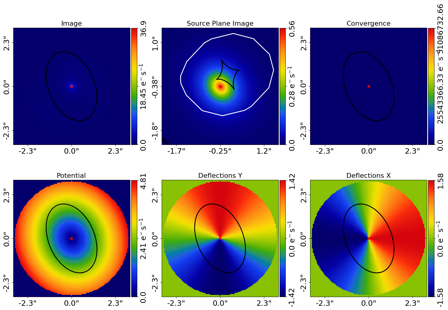
The result also contains the maximum log likelihood Tracer and FitImaging objects which can easily be plotted.
tracer_plotter = aplt.TracerPlotter(
    tracer=result.max_log_likelihood_tracer, grid=dataset.grid
)
tracer_plotter.subplot_tracer()

fit_plotter = aplt.FitImagingPlotter(fit=result.max_log_likelihood_fit)
fit_plotter.subplot_fit()
Here’s what the maximum likelihood tracer looks like:
Here’s what the maximum likelihood fit looks like:
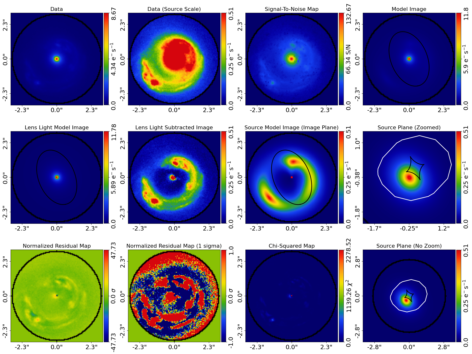
The fit has more significant residuals than the previous tutorial. It is clear that the lens model cannot fully capture the central emission of the lens galaxy and the complex structure of the lensed source galaxy. Nevertheless, it is sufficient to estimate simple lens quantities, like the Einstein Mass. The next examples cover all the features that PyAutoLens has to improve the model-fit.
A full guide of result objects is contained in the autolens_workspace/*/imaging/results package.
Model Customization#
The model can be fully customized, making it simple to parameterize and fit many different lens models using any combination of light and mass profiles.
# Lens:

bulge = af.Model(al.lp.DevVaucouleurs)
mass = af.Model(al.mp.Isothermal)

"""
This aligns the light and mass profile centres in the model, reducing the
number of free parameter fitted for by Dynesty by 2.
"""
bulge.centre = mass.centre

"""
This fixes the lens galaxy light profile's effective radius to a value of
0.8 arc-seconds, removing another free parameter.
"""
bulge.effective_radius = 0.8

"""
This forces the mass profile's einstein radius to be above 1.0 arc-seconds.
"""
mass.add_assertion(lens.mass.einstein_radius > 1.0)

lens = af.Model(
    al.Galaxy,
    redshift=0.5,
    bulge=bulge,
    mass=mass
)
The info attribute shows the customized lens model.
print(lens.info)
This gives the following output:
Total Free Parameters = 8

model                                       Galaxy (N=8)
    bulge                                   DevVaucouleurs (N=5)
    mass                                    Isothermal (N=5)

redshift                                    0.5
bulge
    centre
        centre_0                            GaussianPrior [25], mean = 0.0, sigma = 0.1
        centre_1                            GaussianPrior [26], mean = 0.0, sigma = 0.1
    ell_comps
        ell_comps_0                         GaussianPrior [21], mean = 0.0, sigma = 0.3
        ell_comps_1                         GaussianPrior [22], mean = 0.0, sigma = 0.3
    intensity                               LogUniformPrior [23], lower_limit = 1e-06, upper_limit = 1000000.0
    effective_radius                        0.8
mass
    centre
        centre_0                            GaussianPrior [25], mean = 0.0, sigma = 0.1
        centre_1                            GaussianPrior [26], mean = 0.0, sigma = 0.1
    ell_comps
        ell_comps_0                         GaussianPrior [27], mean = 0.0, sigma = 0.3
        ell_comps_1                         GaussianPrior [28], mean = 0.0, sigma = 0.3
    einstein_radius                         UniformPrior [29], lower_limit = 0.0, upper_limit = 8.0
Model Cookbook#
The readthedocs contain a modeling cookbook which provides a concise reference to all the ways to customize a lens model: https://pyautolens.readthedocs.io/en/latest/general/model_cookbook.html
Linear Light Profiles#
PyAutoLens supports ‘linear light profiles’, where the intensity parameters of all parametric components are solved via linear algebra every time the model is fitted using a process called an inversion. This inversion always computes intensity values that give the best fit to the data (e.g. they maximize the likelihood) given the other parameter values of the light profile.
The intensity parameter of each light profile is therefore not a free parameter in the model-fit, reducing the dimensionality of non-linear parameter space by the number of light profiles (in the example below by 3) and removing the degeneracies that occur between the intensity and other light profile parameters (e.g. effective_radius, sersic_index).
For complex models, linear light profiles are a powerful way to simplify the parameter space to ensure the best-fit model is inferred.
A full descriptions of this feature is given in the linear_light_profiles example:
Multi Gaussian Expansion#
A natural extension of linear light profiles are basis functions, which group many linear light profiles together in order to capture complex and irregular structures in a galaxy’s emission.
Using a clever model parameterization a basis can be composed which corresponds to just N = 4-6 parameters, making model-fitting efficient and robust.
A full descriptions of this feature is given in the multi_gaussian_expansion example:
Shapelets#
PyAutoLens also supports Shapelets, which are a powerful way to fit the light of the galaxies which typically act as the source galaxy in strong lensing systems.
A full descriptions of this feature is given in the shapelets example:
Pixelizations#
The source galaxy can be reconstructed using adaptive pixel-grids (e.g. a Voronoi mesh or Delaunay triangulation), which unlike light profiles, a multi Gaussian expansion or shapelets are not analytic functions that conform to certain symmetric profiles.
This means they can reconstruct more complex source morphologies and are better suited to performing detailed analyses of a lens galaxy’s mass.
A full descriptions of this feature is given in the pixelization example:
The fifth overview example of the readthedocs also give a description of pixelizations:
https://pyautolens.readthedocs.io/en/latest/overview/images/overview_5_pixelizations.html
Wrap-Up#
A more detailed description of lens modeling is provided at the following example:
Chapters 2 and 3 HowToLens lecture series give a comprehensive description of lens modeling, including a description of what a non-linear search is and strategies to fit complex lens model to data in efficient and robust ways.