Interferometry

PyAutoLens supports modeling of interferometer data from submillimeter and radio observatories such as ALMA or LOFAR.

The visibilities of the interferometer dataset are fitted directly in the uv-plane, circumventing issues that arise when fitting a dirty image produced via the visibilities.

The most important issue this addresses is removing correlated noise from impacting the fit.

Real Space Mask

To begin, we define a real-space mask. Although interferometer lens modeling is performed in the uv-plane and therefore Fourier space, we still need to define the grid of coordinates in real-space from which the lensed source’s images are computed. It is this image that is mapped to Fourier space to compare to the uv-plane data.

The size and resolution of this mask depend on the baselines of your interferometer dataset. datasets with longer baselines (i.e. higher resolution data) require higher resolution and larger masks.

import autolens as al
import autolens.plot as aplt

real_space_mask_2d = ag.Mask2D.circular(
    shape_native=(400, 400), pixel_scales=0.025, radius=3.0
)

Interferometer Data

We next load an interferometer dataset from fits files, which follows the same API that we have seen for an Imaging object.

dataset_path = "/path/to/dataset/folder"

dataset = al.Interferometer.from_fits(
    data_path=path.join(dataset_path, "data.fits"),
    noise_map_path=path.join(dataset_path, "noise_map.fits"),
    uv_wavelengths_path=path.join(dataset_path, "uv_wavelengths.fits"),
    real_space_mask=real_space_mask_2d
)

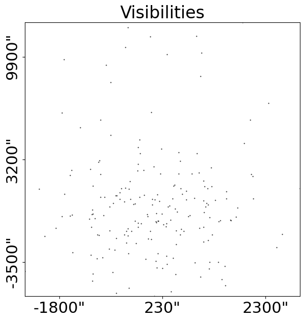
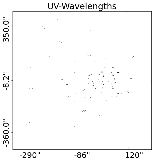
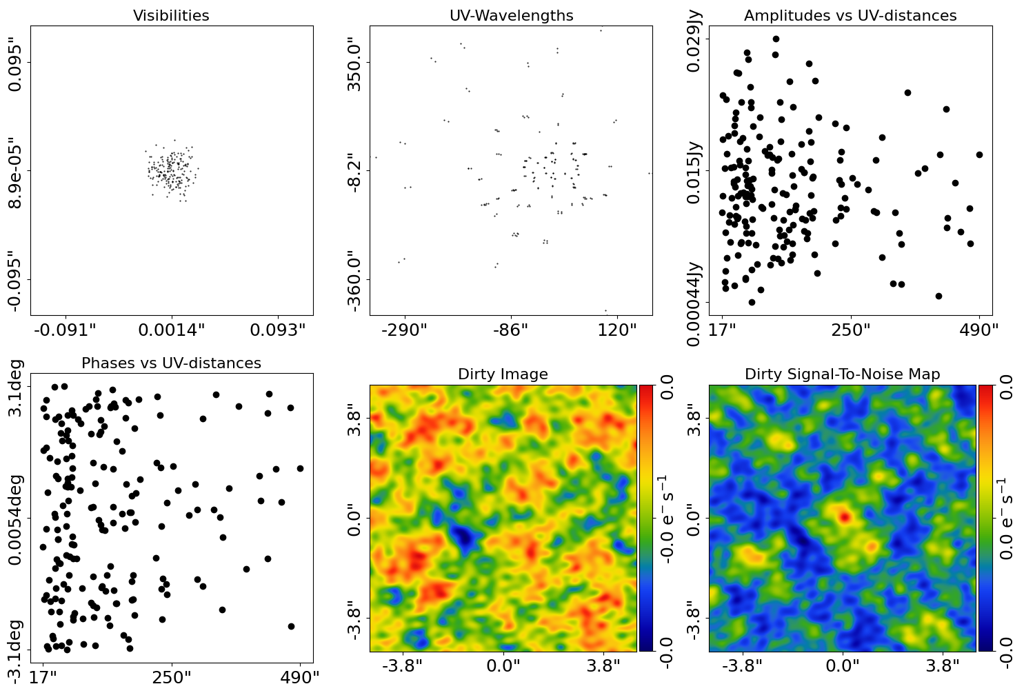
The PyAutoLens plot module has tools for plotting interferometer datasets, including the visibilities, noise-map and uv wavelength which represent the interferometer’s baselines.

The data used in this tutorial contains only ~300 visibilities and is representative of a low resolution Square-Mile Array (SMA) dataset.

We made this choice so the script runs fast, and we discuss below how PyAutoLens can scale up to large visibilities datasets from an instrument like ALMA.

dataset_plotter = aplt.InterferometerPlotter(dataset=dataset)
dataset_plotter.figures_2d(data=True, uv_wavelengths=True)

Here is what the interferometer visibilities and uv wavelength (which represent the interferometer’s baselines):

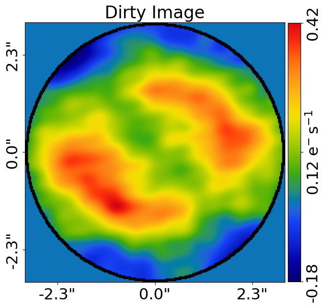
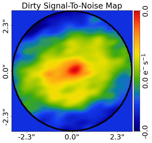
It can also plot dirty images of the dataset in real-space, using the fast Fourier transforms described below.

dataset_plotter = aplt.InterferometerPlotter(interferometer=interferometer)
dataset_plotter.figures_2d(dirty_image=True, dirty_signal_to_noise_map=True)

Here is what the image and signal-to-noise map look like in real space:

Tracer

To perform uv-plane modeling, PyAutoLens generates an image of the strong lens system in real-space via a tracer.

Lets quickly set up the Tracer we’ll use in this example.

lens_galaxy = al.Galaxy(
    redshift=0.5,
    mass=al.mp.Isothermal(
        centre=(0.0, 0.0),
        einstein_radius=1.6,
        ell_comps=al.convert.ell_comps_from(axis_ratio=0.9, angle=45.0),
    ),
    shear=al.mp.ExternalShear(gamma_1=0.05, gamma_2=0.05),
)

source_galaxy = al.Galaxy(
    redshift=1.0,
    bulge=al.lp.Sersic(
        centre=(0.0, 0.0),
        ell_comps=al.convert.ell_comps_from(axis_ratio=0.8, angle=60.0),
        intensity=0.3,
        effective_radius=1.0,
        sersic_index=2.5,
    ),
)

tracer = al.Tracer.from_galaxies(galaxies=[lens_galaxy, source_galaxy])

tracer_plotter = aplt.TracerPlotter(
    tracer=tracer, grid=real_space_mask.derive_grid.unmasked_sub_1
)
tracer_plotter.figures_2d(image=True)

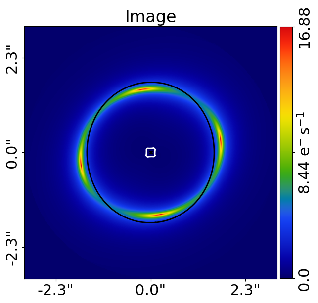
Here is what the image of the tracer looks like:

UV-Plane FFT

To perform uv-plane modeling, PyAutoLens next Fourier transforms this image from real-space to the uv-plane.

This operation uses a Transformer object, of which there are multiple available in PyAutoLens. This includes a direct Fourier transform which performs the exact Fourier transform without approximation.

transformer_class = al.TransformerDFT

However, the direct Fourier transform is inefficient. For ~10 million visibilities, it requires thousands of seconds to perform a single transform. This approach is therefore unfeasible for high quality ALMA and radio datasets.

For this reason, PyAutoLens supports the non-uniform fast fourier transform algorithm PyNUFFT (https://github.com/jyhmiinlin/pynufft), which is significantly faster, being able to perform a Fourier transform of ~10 million in less than a second!

transformer_class = al.TransformerNUFFT

To use this transformer in a fit, we use the apply_settings method.

dataset = dataset.apply_settings(
    settings=al.SettingsInterferometer(transformer_class=transformer_class)
)

Fitting

The interferometer can now be passed to a FitInterferometer object to fit it to a dataset:

fit = al.FitInterferometer(
    interferometer=interferometer, tracer=tracer
)

Visualization of the fit is provided both in the uv-plane and in real-space.

Note that the fit is not performed in real-space, but plotting it in real-space is often more informative.

fit = al.FitInterferometer(
    interferometer=interferometer, tracer=tracer
)

fit_plotter = aplt.FitInterferometerPlotter(fit=fit)
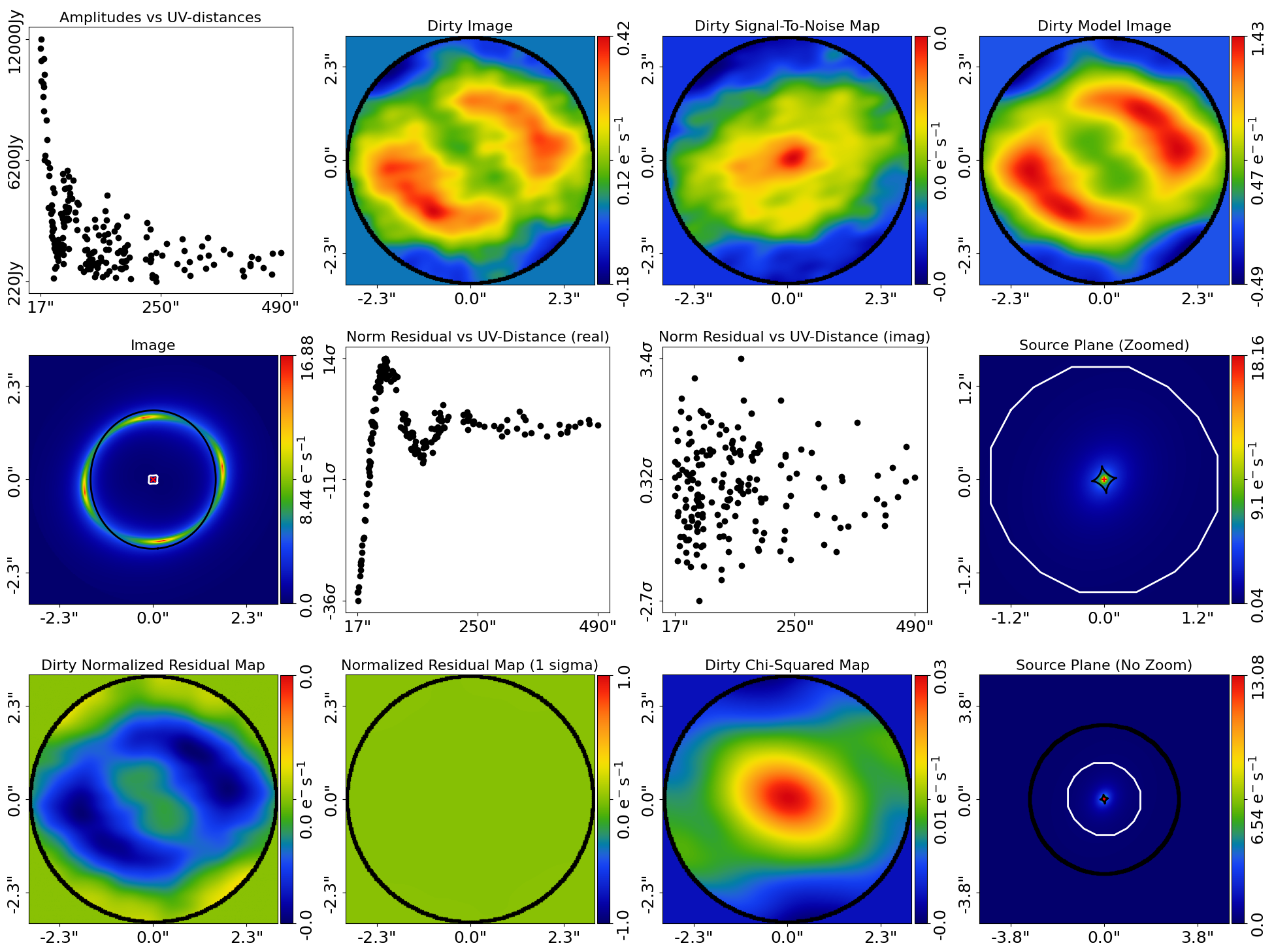
fit_plotter.subplot_fit()

Here is what the subplot image looks like:

Pixelized Sources

Interferometer data can also be modeled using pixelized source’s, which again performs the source reconstruction by directly fitting the visibilities in the uv-plane.

pixelization = al.Pixelization(
    mesh=al.mesh.DelaunayMagnification(shape=(30, 30)),
    regularization=al.reg.Constant(coefficient=1.0),
)

source_galaxy = al.Galaxy(redshift=1.0, pixelization=pixelization)

tracer = al.Tracer.from_galaxies(galaxies=[lens_galaxy, source_galaxy])

fit = al.FitInterferometer(
    dataset=dataset,
    tracer=tracer,
    settings_inversion=al.SettingsInversion(use_linear_operators=True),
)

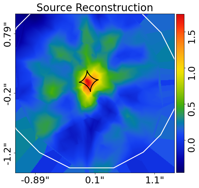
The source reconstruction is visualized in real space:

fit_plotter = aplt.FitInterferometerPlotter(fit=fit)
fit_plotter.figures_2d_of_planes(plane_index=1, plane_image=True)

Here is what it looks like:

Computing this source reconstruction would be extremely inefficient if PyAutoLens used a traditional approach to linear algebra which explicitly stored in memory the values required to solve for the source fluxes. In fact, for an interferometer dataset of ~10 million visibilities this would require hundreds of GB of memory!

PyAutoLens uses the library PyLops (https://pylops.readthedocs.io/en/latest/) to represent this calculation as a sequence of memory-light linear operators.

The combination of PyNUFFT and PyLops makes the analysis of ~10 million visibilities from observatories such as ALMA and JVLA feasible in PyAutoLens.

Lens Modeling

It is straight forward to fit a lens model to an interferometer dataset, using the same API that we saw for imaging data.

We first compose the model, omitted the lens light components given that most strong lenses observed at submm / radio wavelengths do not have visible lens galaxy emission.

# Lens:

mass = af.Model(al.mp.Isothermal)

lens = af.Model(al.Galaxy, redshift=0.5, mass=mass)

# Source:

disk = af.Model(al.lp.Exponential)

source = af.Model(al.Galaxy, redshift=1.0, disk=disk)

# Overall Lens Model:

model = af.Collection(galaxies=af.Collection(lens=lens, source=source))

We again choose the non-linear search dynesty (https://github.com/joshspeagle/dynesty).

search = af.Nautilus(path_prefix="overview", name="interferometer")

Whereas we previously used an AnalysisImaging object, we instead use an AnalysisInterferometer object which fits the lens model in the correct way for an interferometer dataset.

This includes mapping the lens model from real-space to the uv-plane via the Fourier transform discussed above.

analysis = al.AnalysisInterferometer(dataset=dataset)

We can now begin the model-fit by passing the model and analysis object to the search, which performs a non-linear search to find which models fit the data with the highest likelihood.

The results can be found in the output/overview_interferometer folder in the autolens_workspace.

result = search.fit(model=model, analysis=analysis)

The PyAutoLens visualization library and FitInterferometer object includes specific methods for plotting the results, for example the maximum log likelihood fit:

fit_plotter = aplt.FitInterferometerPlotter(fit=result.max_log_likelihood_fit)
fit_plotter.subplot_fit()

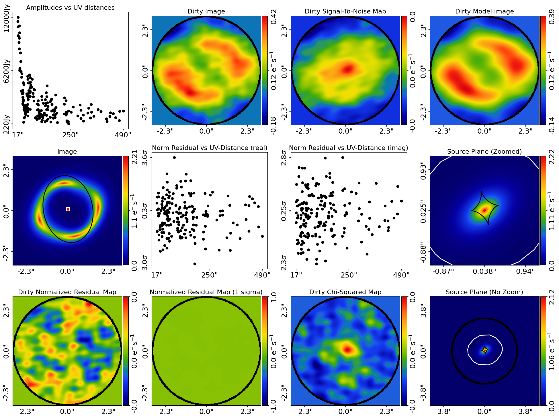
Here is what it looks like:

Simulations

Simulated interferometer datasets can be generated using the SimulatorInterferometer object, which includes adding Gaussian noise to the visibilities:

simulator = al.SimulatorInterferometer(
    uv_wavelengths=dataset.uv_wavelengths, exposure_time=300.0, noise_sigma=0.01
)

real_space_grid = al.Grid2D.uniform(
    shape_native=real_space_mask.shape_native,
    pixel_scales=real_space_mask.pixel_scales,
)

dataset = simulator.via_tracer_from(tracer=tracer, grid=real_space_grid)

dataset_plotter = aplt.InterferometerPlotter(dataset=dataset)
dataset_plotter.subplot_dataset()

Here is the subplot of the simulated interferometer dataset:

Wrap-Up

The interferometer package of the autolens_workspace contains numerous example scripts for performing interferometer modeling and simulating strong lens interferometer datasets.