Simulating Lenses#
PyAutoLens provides tool for simulating strong lens data-sets, which can be used to test lens modeling pipelines and train neural networks to recognise and analyse images of strong lenses.
Grid And Lens#
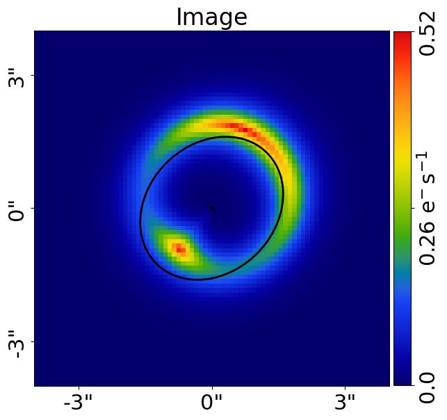
In this overview we use a tracer and grid to create an image of a strong lens.
Everything below has been covered in previous overview examples, so if any code doesn’t make sense you should go back and checkout the appropriate example!
import autolens as al
import autolens.plot as aplt

grid = al.Grid2D.uniform(
    shape_native=(80, 80),
    pixel_scales=0.1,  # <- The pixel-scale describes the conversion from pixel units to arc-seconds.
)

lens_galaxy = al.Galaxy(
    redshift=0.5,
    mass=al.mp.Isothermal(centre=(0.0, 0.0), ell_comps=(0.1, 0.0), einstein_radius=1.6),
)

source_galaxy = al.Galaxy(
    redshift=1.0,
    bulge=al.lp.Exponential(
        centre=(0.3, 0.2),
        ell_comps=(0.1, 0.0),
        intensity=0.1,
        effective_radius=0.5,
    ),
)

tracer = al.Tracer(
    galaxies=[lens_galaxy, source_galaxy], cosmology=al.cosmo.Planck15()
)

tracer_plotter = aplt.TracerPlotter(tracer=tracer, grid=grid)
tracer_plotter.figures_2d(image=True)
Simulator#
Simulating strong lens images uses a SimulatorImaging object, which simulates the process that an instrument like the
Hubble Space Telescope goes through when it acquires imaging of a strong lens, including:
Using for the exposure time to determine the signal-to-noise of the data by converting the simulated image from electrons per second to electrons.
Blurring the observed light of the strong lens with the telescope optics via its point spread function (psf).
Accounting for the background sky in the exposure which adds Poisson noise.
psf = al.Kernel2D.from_gaussian(shape_native=(11, 11), sigma=0.1, pixel_scales=0.05)

simulator = al.SimulatorImaging(
    exposure_time=300.0, background_sky_level=1.0, psf=psf, add_poisson_noise=True
)
Once we have a simulator, we can use it to create an imaging dataset which consists of image data, a noise-map and a Point Spread Function (PSF).
We do this by passing it a tracer and grid, where it uses the tracer above to create the image of the strong lens and then add the effects that occur during data acquisition.
dataset = simulator.from_tracer_and_grid(tracer=tracer, grid=grid)
By plotting a subplot of the Imaging dataset, we can see this object includes the observed image of the strong lens
(which has had noise and other instrumental effects added to it) as well as a noise-map and PSF:
dataset_plotter = aplt.ImagingPlotter(dataset=dataset)
dataset_plotter.subplot_dataset()
Here is what the dataset looks like:
Examples#
The autolens_workspace includes many example simulators for simulating strong lenses with a range of different
physical properties and for creating imaging datasets for a variety of telescopes (e.g. Hubble, Euclid).
Below, we show what a strong lens looks like for different instruments.
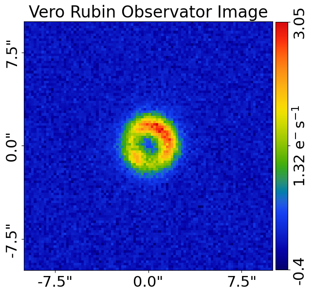

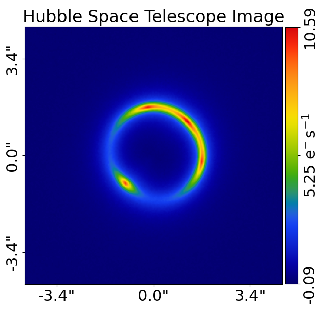

Wrap Up#
The autolens_workspace includes many example simulators for simulating strong lenses with a range of different physical properties, for example lenses without any lens light, with multiple lens galaxies, and double Einstein ring lenses.
There are also tools for making datasets for a variety of telescopes (e.g. Hubble, Euclid) and interferometer datasets (e.g. ALMA).