Multi-Wavelength#
PyAutoLens supports the analysis of multiple datasets simultaneously, including many CCD imaging datasets observed at different wavebands (e.g. red, blue, green) and combining imaging and interferometer datasets.
This enables multi-wavelength lens modeling, where the color of the lens and source galaxies vary across the datasets.
Multi-wavelength lens modeling offers a number of advantages:
It provides a wealth of additional information to fit the lens model, especially if the source changes its appearance across wavelength.
It overcomes challenges associated with the lens and source galaxy emission blending with one another, as their brightness depends differently on wavelength.
Instrument systematic effects, for example an uncertain PSF, will impact the model less because they vary across each dataset.
Multi-Wavelength Imaging#
For multi-wavelength imaging datasets, we begin by defining the colors of the multi-wavelength images.
For this overview we use only two colors, green (g-band) and red (r-band), but extending this to more datasets is straight forward.
import autolens as al
import autolens.plot as aplt

color_list = ["g", "r"]
Every dataset in our multi-wavelength observations can have its own unique pixel-scale.
pixel_scales_list = [0.08, 0.12]
Multi-wavelength imaging datasets do not use any new objects or class in PyAutoLens.
We simply use lists of the classes we are now familiar with, for example the Imaging class.
dataset_path = path.join("dataset", "multi", "imaging", "lens_sersic")

dataset_list = [
    al.Imaging.from_fits(
        image_path=path.join(dataset_path, f"{color}_image.fits"),
        psf_path=path.join(dataset_path, f"{color}_psf.fits"),
        noise_map_path=path.join(dataset_path, f"{color}_noise_map.fits"),
        pixel_scales=pixel_scales,
    )
    for color, pixel_scales in zip(color_list, pixel_scales_list)]
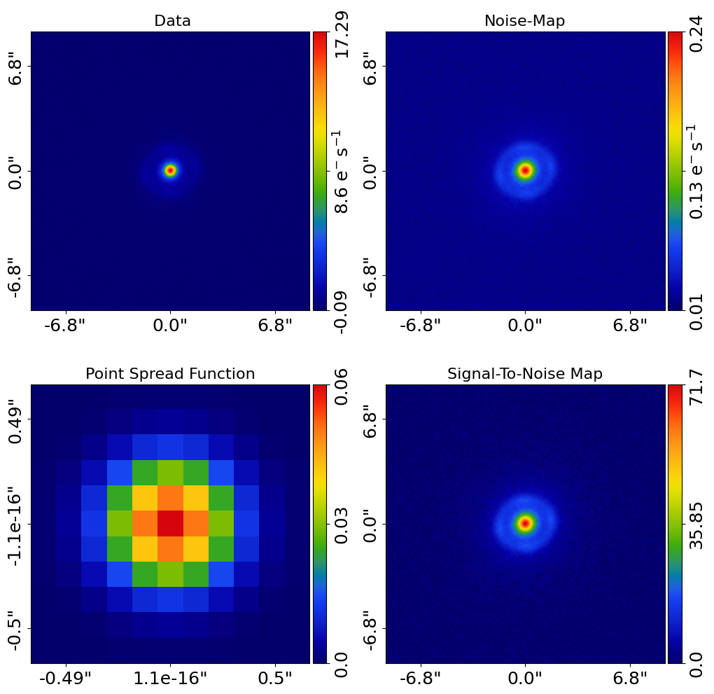
Here is what our r-band and g-band observations of this lens system looks like.
In the r-band, the lens outshines the source, whereas in the g-band the source galaxy is more visible.
The different variation of the colors of the lens and source across wavelength is a powerful tool for lens modeling, as it helps deblend the two objects.
for dataset in dataset_list:

    dataset_plotter = aplt.ImagingPlotter(dataset=dataset)
    dataset_plotter.subplot_dataset()
Here are the g-band images:
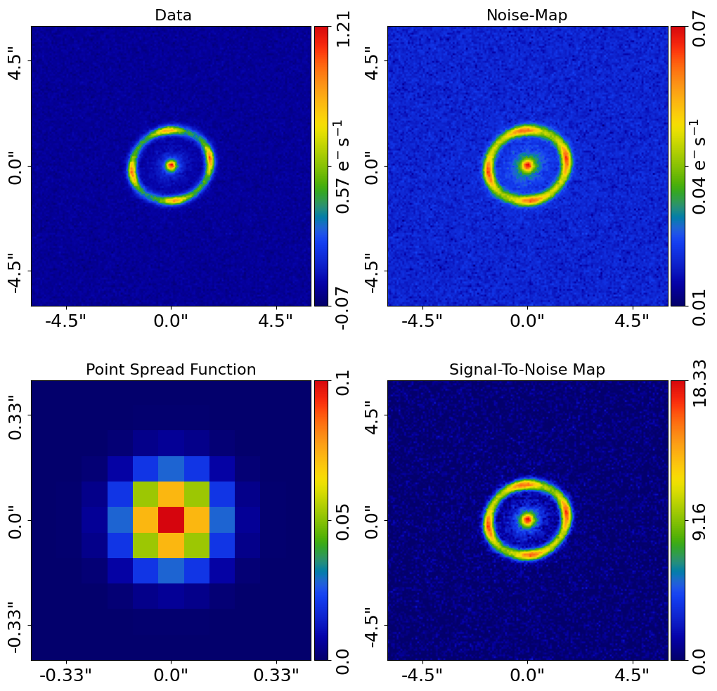
Here are the r-band images:
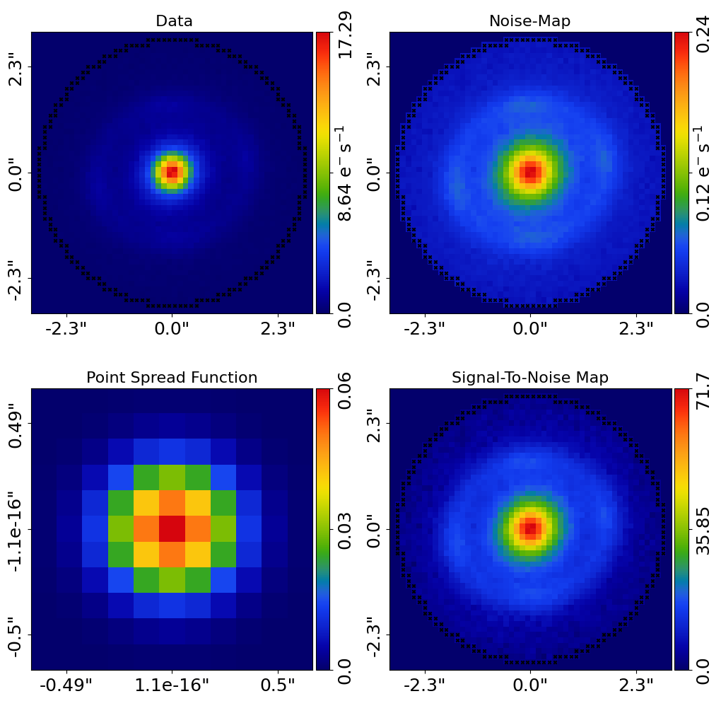
Define a 3.0” circular mask, which includes the emission of the lens and source galaxies.
For multi-wavelength lens modeling, we use the same mask for every dataset whenever possible. This is not absolutely necessary, but provides a more reliable analysis.
mask_2d_list = [
    al.Mask2D.circular(
        shape_native=dataset.shape_native, pixel_scales=dataset.pixel_scales, radius=3.0
    )
    for dataset in dataset_list
]

dataset_list = [
dataset.apply_mask(mask=mask) for dataset, mask in zip(dataset_list, mask_list)
]
- for dataset in dataset_list:
dataset_plotter = aplt.ImagingPlotter(dataset=dataset) dataset_plotter.subplot_dataset()
Here is how the masked g-band dataset appears:
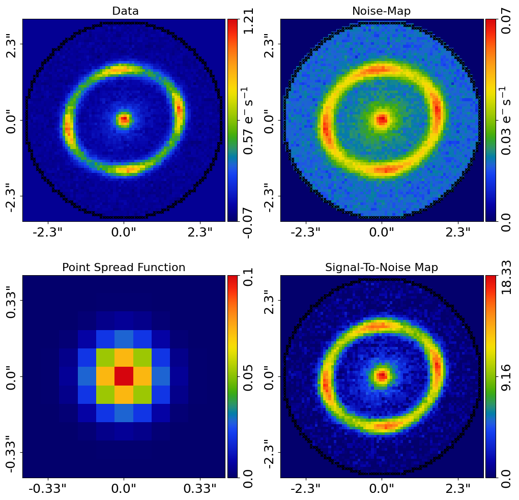
Here is how the masked r-band dataset appears:
Analysis#
We create a list of AnalysisImaging objects for every dataset.
analysis_list = [al.AnalysisImaging(dataset=dataset) for dataset in dataset_list]
We now introduce the key new aspect to the PyAutoLens multi-dataset API, which is critical to fitting multiple datasets simultaneously.
We sum the list of analysis objects to create an overall CombinedAnalysis object, which we can use to fit the
multi-wavelength imaging data, where:
The log likelihood function of this summed analysis class is the sum of the log likelihood functions of each individual analysis objects (e.g. the fit to each separate waveband).
The summing process ensures that tasks such as outputting results to hard-disk, visualization, etc use a structure that separates each analysis and therefore each dataset.
analysis = sum(analysis_list)
Model#
We compose an initial lens model as per usual.
# Lens:

bulge = af.Model(al.lp.Sersic)
mass = af.Model(al.mp.Isothermal)
shear = af.Model(al.mp.ExternalShear)

lens = af.Model(
    al.Galaxy,
    redshift=0.5,
    bulge=bulge,
    mass=mass,
    shear=shear,
)

# Source:

bulge = af.Model(al.lp.Sersic)

source = af.Model(al.Galaxy, redshift=1.0, bulge=bulge)

# Overall Lens Model:

model = af.Collection(galaxies=af.Collection(lens=lens, source=source))
However, there is a problem for multi-wavelength datasets. Should the light profiles of the lens’s bulge and source’s bulge have the same parameters for each wavelength image?
The answer is no. At different wavelengths, different stars appear brighter or fainter, meaning that the overall appearance of the lens and source galaxies will change.
We therefore allow specific light profile parameters to vary across wavelength and act as additional free parameters in the fit to each image.
We do this using the combined analysis object as follows:
analysis = analysis.with_free_parameters(
    model.galaxies.lens.bulge.intensity, model.galaxies.source.bulge.intensity
)
In this simple overview, this has added two additional free parameters to the model whereby:
The lens bulge’s intensity is different in both multi-wavelength images.
The source bulge’s intensity is different in both multi-wavelength images.
It is entirely plausible that more parameters should be free to vary across wavelength (e.g. the lens and source
galaxies effective_radius or sersic_index parameters).
This choice ultimately depends on the quality of data being fitted and intended science goal. Regardless, it is clear how the above API can be extended to add any number of additional free parameters.
Result#
Fitting the model uses the same API we introduced in previous overviews.
The result object returned by this model-fit is a list of Result objects, because we used a combined analysis.
Each result corresponds to each analysis created above and is there the fit to each dataset at each wavelength.
search = af.Nautilus(name="overview_example_multiwavelength")
result_list = search.fit(model=model, analysis=analysis)
Plotting each result’s tracer shows that the lens and source galaxies appear different in each result, owning to their different intensities.
for result in result_list:

    tracer_plotter = aplt.TracerPlotter(
        tracer=result.max_log_likelihood_tracer, grid=result.grid
    )
    tracer_plotter.subplot_tracer()
Here is how the g-band subplot appears:
Here is how the r-band subplot appears:
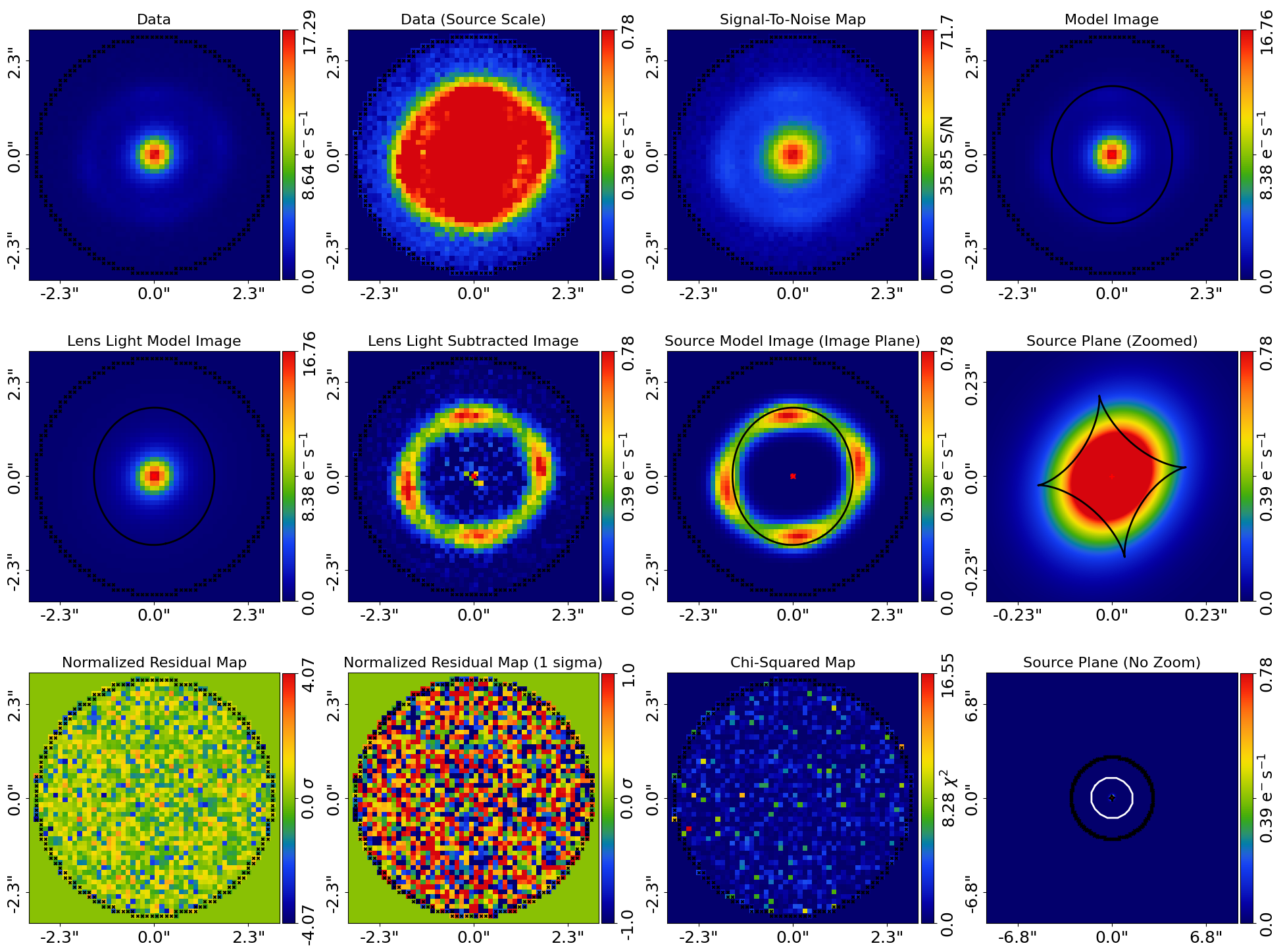
Subplots of each fit show that a good overall fit is achieved to each dataset.
for result in result_list:
    fit_plotter = aplt.FitImagingPlotter(
        fit=result.max_log_likelihood_fit,
    )
    fit_plotter.subplot_fit()
Here is how the g-band subplot appears:
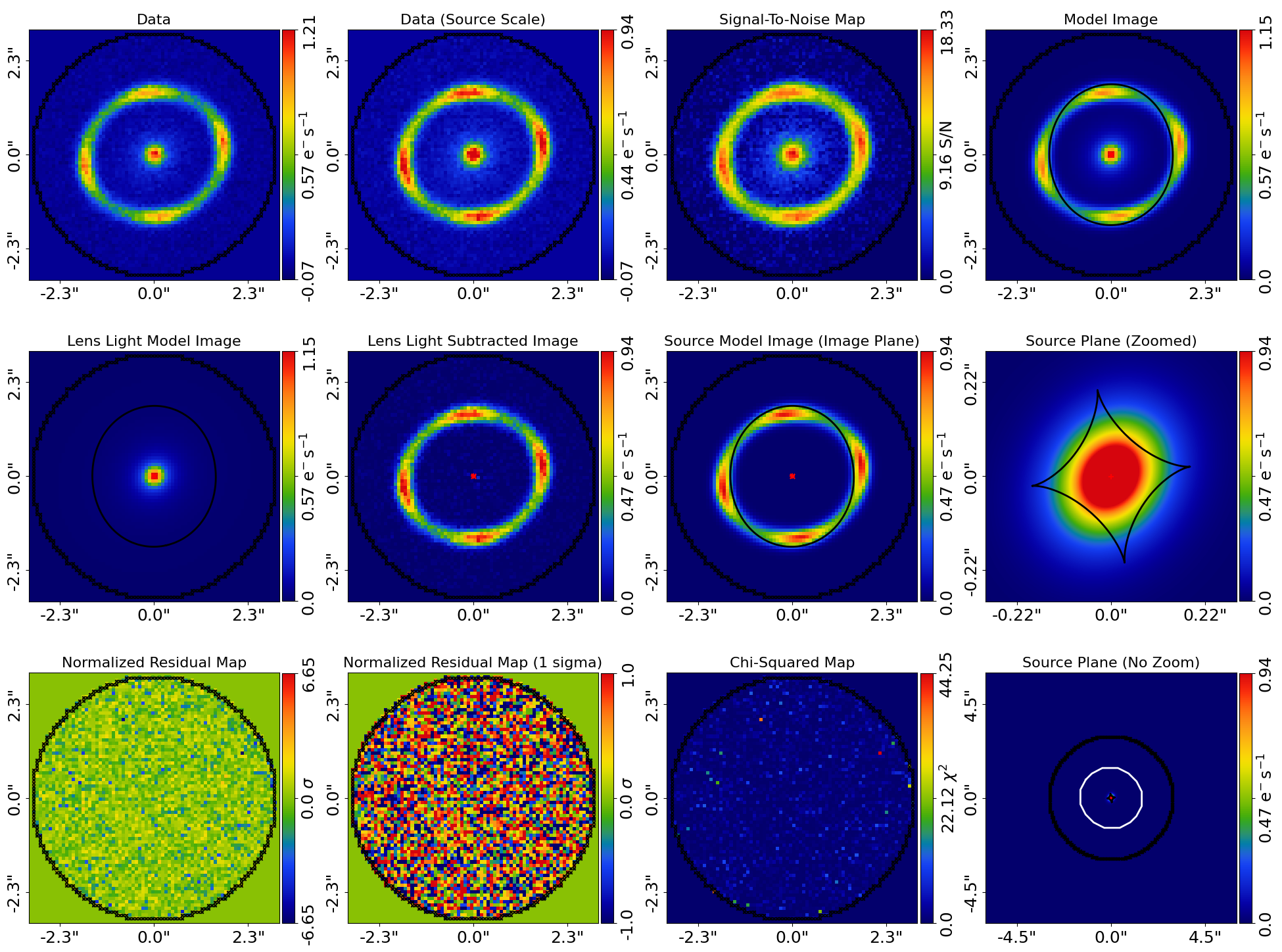
Here is how the r-band subplot appears:
Wavelength Dependence#
In the example above, a free intensity parameter is created for every multi-wavelength dataset. This would add 5+
free parameters to the model if we had 5+ datasets, quickly making a complex model parameterization.
We can instead parameterize the intensity of the lens and source galaxies as a user defined function of
wavelength, for example following a relation y = (m * x) + c -> intensity = (m * wavelength) + c.
By using a linear relation y = mx + c the free parameters are m and c, which does not scale with the number
of datasets. For datasets with multi-wavelength images (e.g. 5 or more) this allows us to parameterize the variation
of parameters across the datasets in a way that does not lead to a very complex parameter space.
Below, we show how one would do this for the intensity of a lens galaxy’s bulge, give three wavelengths corresponding
to a dataset observed in the g and I bands.
wavelength_list = [464, 658, 806]

lens_m = af.UniformPrior(lower_limit=-0.1, upper_limit=0.1)
lens_c = af.UniformPrior(lower_limit=-10.0, upper_limit=10.0)

source_m = af.UniformPrior(lower_limit=-0.1, upper_limit=0.1)
source_c = af.UniformPrior(lower_limit=-10.0, upper_limit=10.0)

analysis_list = []

for wavelength, dataset in zip(wavelength_list, dataset_list):

    lens_intensity = (wavelength * lens_m) + lens_c
    source_intensity = (wavelength * source_m) + source_c

    analysis_list.append(
        al.AnalysisImaging(dataset=dataset).with_model(
            model.replacing(
                {
                    model.galaxies.lens.bulge.intensity: lens_intensity,
                    model.galaxies.source.bulge.intensity: source_intensity,
                }
            )
        )
    )
Same Wavelengths#
The above API can fit multiple datasets which are observed at the same wavelength.
For example, this allows the analysis of images of a galaxy before they are combined to a single frame via the multidrizzling data reduction process to remove correlated noise in the data.
The pointing of each observation, and therefore centering of each dataset, may vary in an unknown way. This can be folded into the model and fitted for as follows.
TODO : add example
Interferometry and Imaging#
The above API can combine modeling of imaging and interferometer datasets (see the autolens_workspace for examples
script showing this in full).
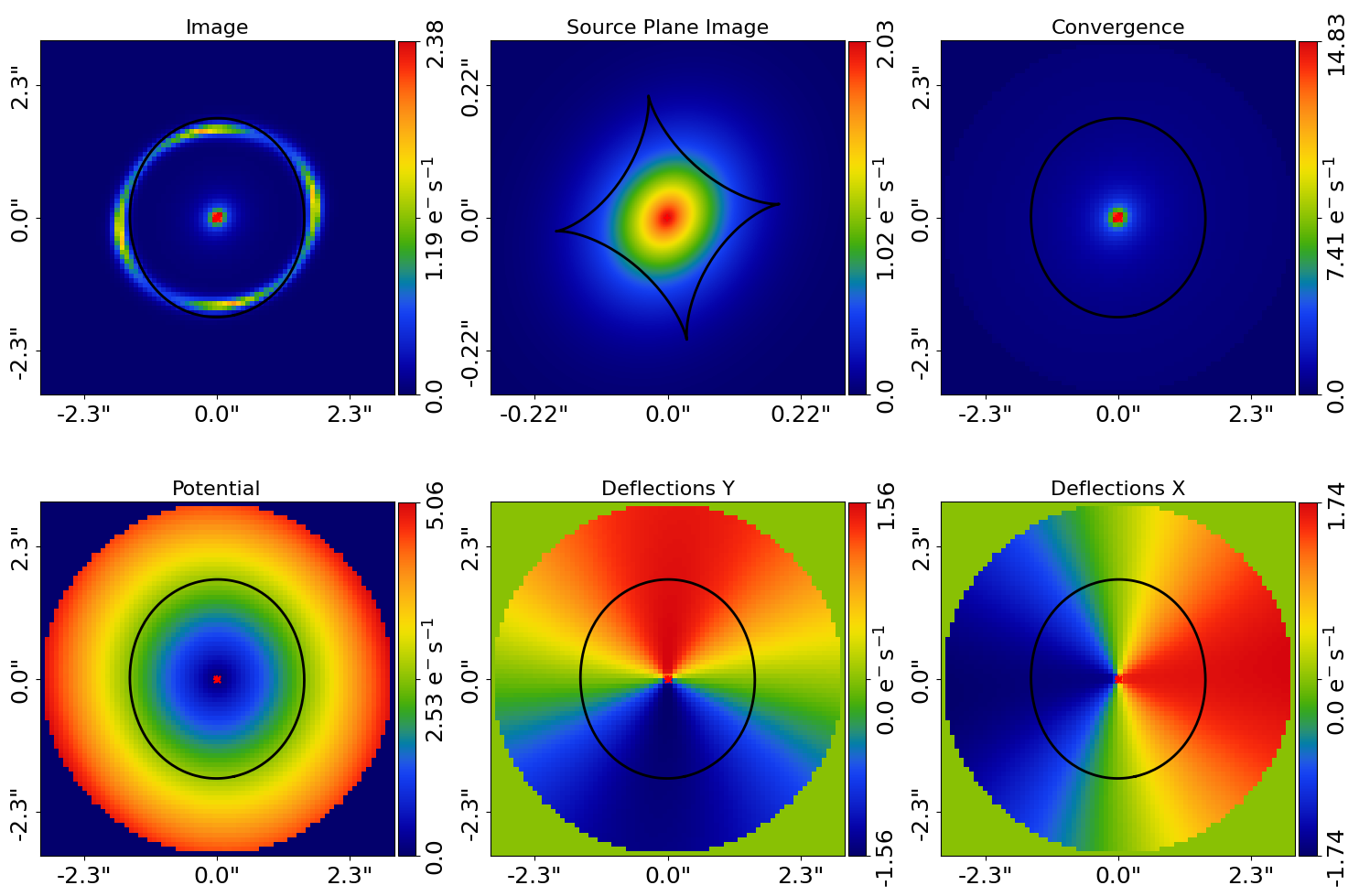
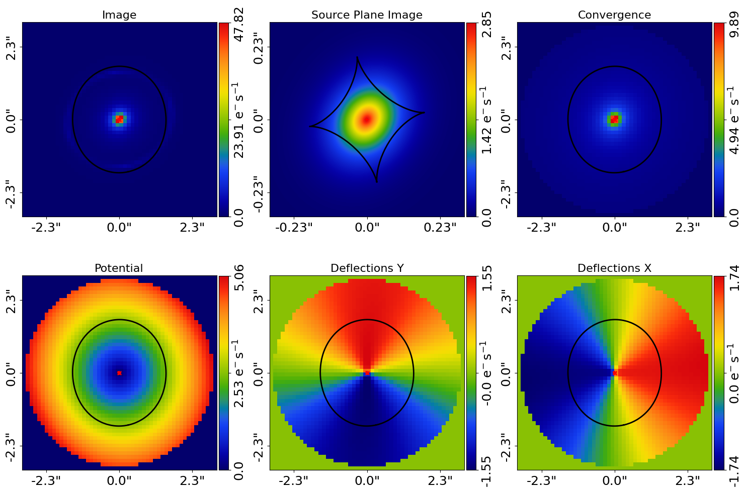
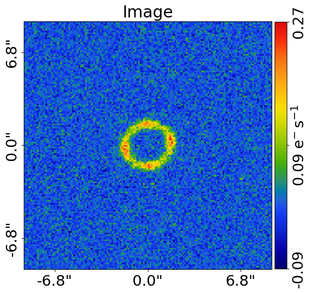
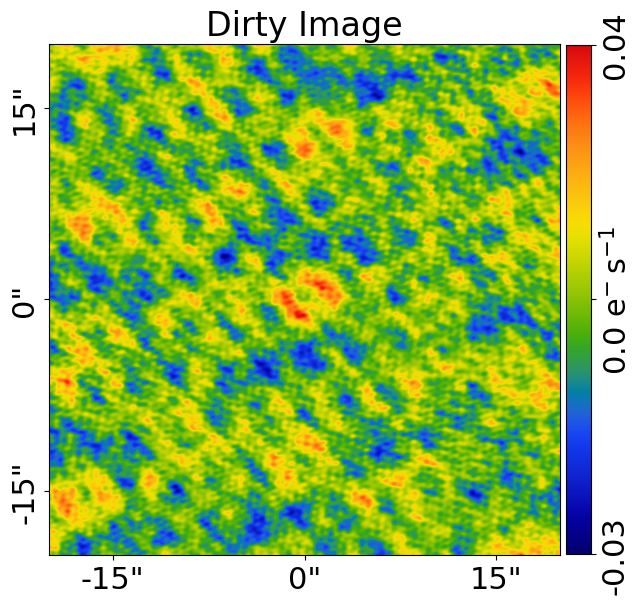
Below are mock strong lens images of a system observed at a green wavelength (g-band) and with an interferometer at sub millimeter wavelengths.
A number of benefits are apparent if we combine the analysis of both datasets at both wavelengths:
The lens galaxy is invisible at sub-mm wavelengths, making it straight-forward to infer a lens mass model by fitting the source at submm wavelengths.
The source galaxy appears completely different in the g-band and at sub-millimeter wavelengths, providing a lot more information with which to constrain the lens galaxy mass model.
Linear Light Profiles#
The modeling overview example described linear light profiles, where the intensity parameters of all parametric
components are solved via linear algebra every time the model is fitted using a process called an inversion.
These profiles are particular powerful when combined with multi-wavelength datasets, because the linear algebra
will solve for the intensity value in each individual dataset separately.
This means that the intensity value of all of the galaxy light profiles in the model vary across the multi-wavelength
datasets, but the dimensionality of the model does not increase as more datasets are fitted.
A full example is given in the linear_light_profiles example:
Wrap-Up#
The multi package of the autolens_workspace contains numerous example scripts for performing multi-wavelength modeling and simulating strong lenses with multiple datasets.