Fitting Data#
A Tracer object represents a strong lens system and allows us to create images of the lens galaxy and lensed source
galaxy.
Loading Data#
We are now going to use a Tracer to fit imaging data of a strong lens, which we begin by loading
from .fits files as an Imaging object:
from os import path

import autolens as al
import autolens.plot as aplt

dataset_name = "simple__no_lens_light"
dataset_path = path.join("dataset", "imaging", dataset_name)

dataset = al.Imaging.from_fits(
    data_path=path.join(dataset_path, "data.fits"),
    psf_path=path.join(dataset_path, "psf.fits"),
    noise_map_path=path.join(dataset_path, "noise_map.fits"),
    pixel_scales=0.1,
)
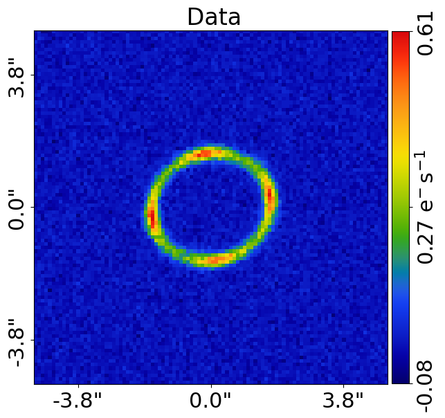
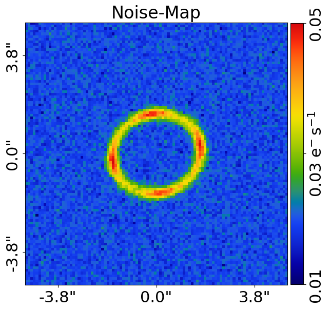
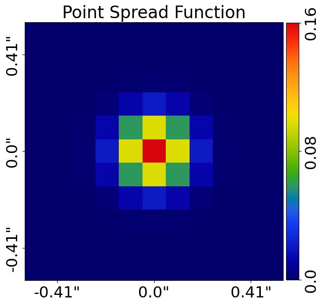
We use the ImagingPlotter to plot the image, noise-map and psf (point-spread function) of the dataset.
dataset_plotter = aplt.ImagingPlotter(dataset=dataset)
dataset_plotter.figures_2d(data=True, noise_map=True, psf=True)
Here’s what our data, noise_map and psf look like:
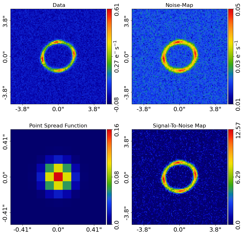
The ImagingPlotter also contains a subplot which plots all these properties simultaneously.
dataset_plotter = aplt.ImagingPlotter(dataset=dataset)
dataset_plotter.subplot_dataset()
Here is what it looks like:
Masking#
We now need to mask the data, so that regions where there is no signal (e.g. the edges) are omitted from the fit.
We use a Mask2D object, which for this example is a 3.0” circular mask.
mask = al.Mask2D.circular(
    shape_native=dataset.shape_native, pixel_scales=dataset.pixel_scales, sub_size=1, radius=3.0
)
We now combine the imaging dataset with the mask:
dataset = dataset.apply_mask(mask=mask_2d)
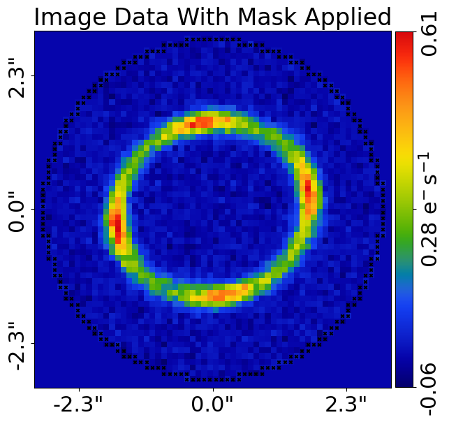
We now plot the image with the mask applied, where the image automatically zooms around the mask to make the lensed source appear bigger. .. code-block:: python
dataset_plotter = aplt.ImagingPlotter(dataset=dataset) dataset_plotter.set_title(“Image Data With Mask Applied”) dataset_plotter.figures_2d(data=True)
Here is what the image looks like:
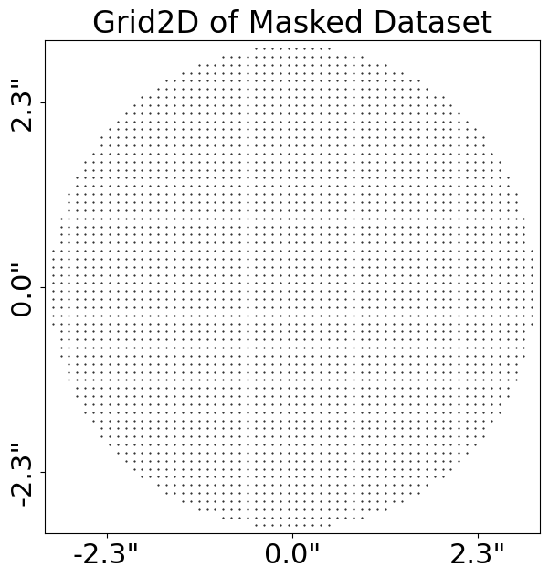
The mask is also used to compute a Grid2D, where the (y,x) arc-second coordinates are only computed in unmasked pixels within the masks’ circle.
As shown in the previous overview example, this grid will be used to perform lensing calculations when fitting the data below.
grid_plotter = aplt.Grid2DPlotter(grid=dataset.grid)
grid_plotter.set_title("Grid2D of Masked Dataset")
grid_plotter.figure_2d()
Here is the grid of the mask:
Fitting#
Following the previous overview example, we can make a tracer from a collection of LightProfile, MassProfile and Galaxy objects.
The combination of LightProfile’s and MassProfile’s below is the same as those used to generate the simulated dataset we loaded above.
It therefore produces a tracer whose image looks exactly like the dataset.
lens_galaxy = al.Galaxy(
    redshift=0.5,
    mass=al.mp.Isothermal(
        centre=(0.0, 0.0),
        einstein_radius=1.6,
        ell_comps=al.convert.ell_comps_from(axis_ratio=0.9, angle=45.0),
    ),
    shear=al.mp.ExternalShear(gamma_1=0.05, gamma_2=0.05),
)

source_galaxy = al.Galaxy(
    redshift=1.0,
    bulge=al.lp.Sersic(
        centre=(0.0, 0.0),
        ell_comps=al.convert.ell_comps_from(axis_ratio=0.8, angle=60.0),
        intensity=0.3,
        effective_radius=0.1,
        sersic_index=1.0,
    ),
)

tracer = al.Tracer(galaxies=[lens_galaxy, source_galaxy])
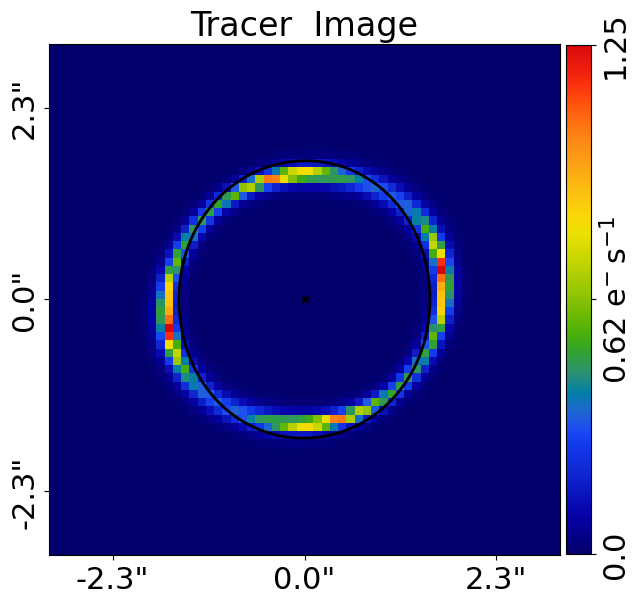
Because the tracer’s light and mass profiles are the same used to make the dataset, its image is nearly the same as the observed image.
However, the tracer’s image does appear different to the data, in that its ring appears a bit thinner. This is because its image has not been blurred with the telescope optics PSF, which the data has.
[For those not familiar with Astronomy data, the PSF describes how the observed emission of the galaxy is blurred by the telescope optics when it is observed. It mimics this blurring effect via a 2D convolution operation].
tracer_plotter = aplt.TracerPlotter(tracer=tracer, grid=dataset.grid)
tracer_plotter.set_title("Tracer`s Image")
tracer_plotter.figures_2d(image=True)
Here is the tracer’s image, which is similar to the dataset shown above:
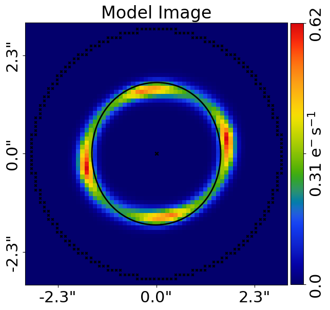
We now use a FitImaging object to fit this tracer to the dataset.
The fit creates a model_image which we fit the data with, which includes performing the step of blurring the tracer`s image with the imaging dataset’s PSF. We can see this by comparing the tracer`s image (which isn’t PSF convolved) and the fit`s model image (which is).
fit = al.FitImaging(dataset=dataset, tracer=tracer)

fit_plotter = aplt.FitImagingPlotter(fit=fit)
fit_plotter.figures_2d(model_image=True)
Here is how the FitImaging’s model-image looks, note how the model-image is thicker than the tracer’s image above
because it has been blurred with the PSF:
The fit does a lot more than just blur the tracer’s image with the PSF, it also creates the following:
The
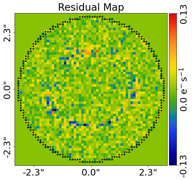
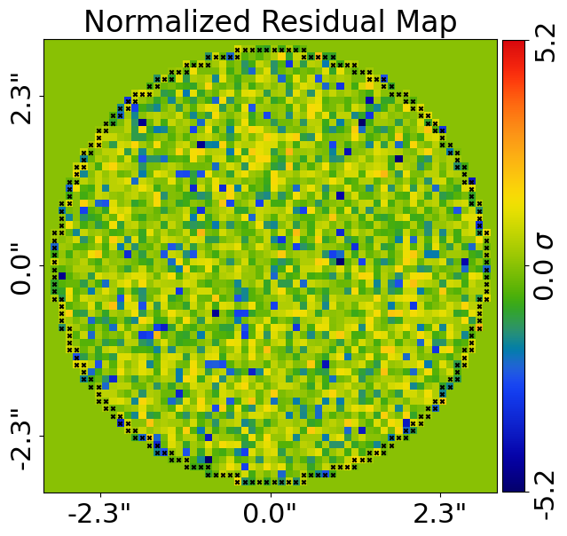
residual_map: Themodel_imagesubtracted from the observed dataset``sdata.The
normalized_residual_map: Theresidual_map ``divided by the observed dataset's ``noise_map.The
chi_squared_map: Thenormalized_residual_mapsquared.
For a good lens model where the model image and tracer are representative of the strong lens system the residuals, normalized residuals and chi-squareds are minimized:
fit_plotter = aplt.FitImagingPlotter(fit=fit)
fit_plotter.figures_2d(
    residual_map=True, normalized_residual_map=True, chi_squared_map=True
)
For a good lens model where the Tracer’s model image is representative of the strong lens system the residuals,
normalized residuals and chi-squared values minimized:

A subplot can be plotted which contains all of the above quantities, as well as other information contained in the tracer such as the source-plane image, a zoom in of the source-plane and a normalized residual map where the colorbar goes from 1.0 sigma to -1.0 sigma, to highlight regions where the fit is poor.
This subplot is probably the most important visualization output by PyAutoLens, and is something you should anticipate seeing a lot of!
fit_plotter.subplot_fit()
Here is the subplot:

Most importantly, the FitImaging object also provides us with a log_likelihood, a single value quantifying
how good the tracer fitted the dataset.
Lens modeling, describe in the next overview example, effectively tries to maximize this log likelihood value.
print(fit.log_likelihood)
Bad Fit#
A bad lens model will show features in the residual-map and chi-squared map.
We can produce such an image by creating a tracer with different lens and source galaxies. In the example below, we change the centre of the source galaxy from (0.0, 0.0) to (0.05, 0.05), which leads to residuals appearing in the fit.
lens_galaxy = al.Galaxy(
    redshift=0.5,
    mass=al.mp.Isothermal(
        centre=(0.0, 0.0),
        einstein_radius=1.6,
        ell_comps=al.convert.ell_comps_from(axis_ratio=0.9, angle=45.0),
    ),
    shear=al.mp.ExternalShear(gamma_1=0.05, gamma_2=0.05),
)

source_galaxy = al.Galaxy(
    redshift=1.0,
    bulge=al.lp.Sersic(
        centre=(0.1, 0.1),
        ell_comps=al.convert.ell_comps_from(axis_ratio=0.8, angle=60.0),
        intensity=0.3,
        effective_radius=0.1,
        sersic_index=1.0,
    ),
)

tracer = al.Tracer(galaxies=[lens_galaxy, source_galaxy])
A new fit using this plane shows residuals, normalized residuals and chi-squared which are non-zero.
fit = al.FitImaging(dataset=dataset, tracer=tracer)

fit_plotter = aplt.FitImagingPlotter(fit=fit)
fit_plotter.subplot_fit()
Here is what this bad fit looks like:
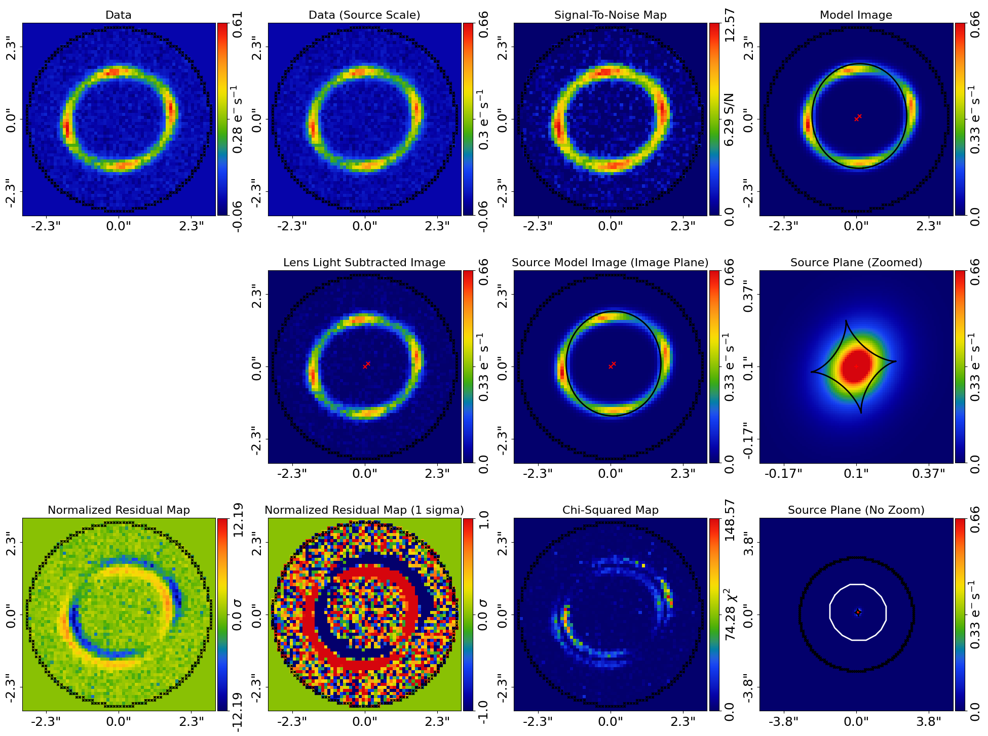
Its log_likelihood is also significantly lower than the good fit above!
Wrap Up#
If you are unfamiliar with data and model fitting, and unsure what terms like ‘residuals’, ‘chi-squared’ or ‘likelihood’ mean, we’ll explain all in chapter 1 of the HowToLens lecture series. Checkout the tutorials section of the readthedocs!