Pixelized Sources#
- Many strongly lensed source galaxies are complex, and they have asymmetric and irregular morphologies. These
morphologies cannot be well approximated by parametric light profiles like a Sersic, or multiple Sersics. Even techniques like a multi-Gaussian expansion or shapelets cannot capture the most complex of source morphologies.
A pixelization reconstructs the source’s light using an adaptive pixel-grid, where the solution is regularized using a prior that forces the solution to have a degree of smoothness.
This means they can reconstruct more complex source morphologies and are better suited to performing detailed analyses of a lens galaxy’s mass.
Dataset#
We load the imaging data that we’ll reconstruct the lensed source galaxy’s light of using a pixelization.
Note how complex the lensed source galaxy looks, with multiple clumps of light. This would be very difficult to model using light profiles!
import autolens as al
import autolens.plot as aplt

dataset_name = "source_complex"
dataset_path = path.join("dataset", "imaging", dataset_name)

dataset = al.Imaging.from_fits(
    data_path=path.join(dataset_path, "data.fits"),
    psf_path=path.join(dataset_path, "psf.fits"),
    noise_map_path=path.join(dataset_path, "noise_map.fits"),
    pixel_scales=0.05,
)

dataset_plotter = aplt.ImagingPlotter(dataset=dataset)
dataset_plotter.subplot_dataset()
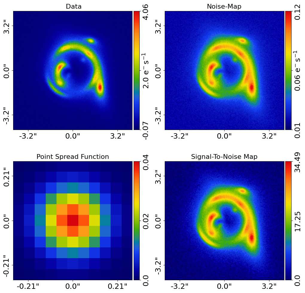
We are going to fit this data via a pixelization, which requires us to define a 2D mask within which the pixelization reconstructs the data.
mask = al.Mask2D.circular(
    shape_native=dataset.shape_native, pixel_scales=dataset.pixel_scales, radius=3.6
)

dataset = dataset.apply_mask(mask=mask)
Rectangular Example#
To reconstruct the source on a pixel-grid, called a mesh, we simply pass it the Mesh class we want to reconstruct its
light. We also pass it a Regularization scheme, describing a prior on how smooth the source reconstruction should be.
Lets use a Rectangular mesh with resolution 40 x 40 pixels and Constant regularizaton scheme with a
regularization coefficient of 1.0. The higher this coefficient, the more our source reconstruction is smoothed.
The isothermal mass model defined below is true model used to simulate the data.
lens_galaxy = al.Galaxy(
    redshift=0.5,
    mass=al.mp.Isothermal(
        centre=(0.0, 0.0), einstein_radius=1.6, ell_comps=(0.17647, 0.0)
    ),
)

pixelization = al.Pixelization(
    mesh=al.mesh.Rectangular(shape=(40, 40)),
    regularization=al.reg.Constant(coefficient=1.0),
)

source_galaxy = al.Galaxy(redshift=1.0, pixelization=pixelization)
Now that our source-galaxy has a Pixelization, we are able to fit the data using the same tools described in
a previous overview example.
We simply pass the source galaxy to a Tracer and using this Tracer to create a FitImaging object.
tracer = al.Tracer(galaxies=[lens_galaxy, source_galaxy])

fit = al.FitImaging(dataset=dataset, tracer=tracer)
The fit has been performed using a pixelization for the source galaxy.
We can see this by plotting the source-plane of the FitImaging using the subplot_fit method.
fit_plotter = aplt.FitImagingPlotter(fit=fit)
fit_plotter.subplot_fit()
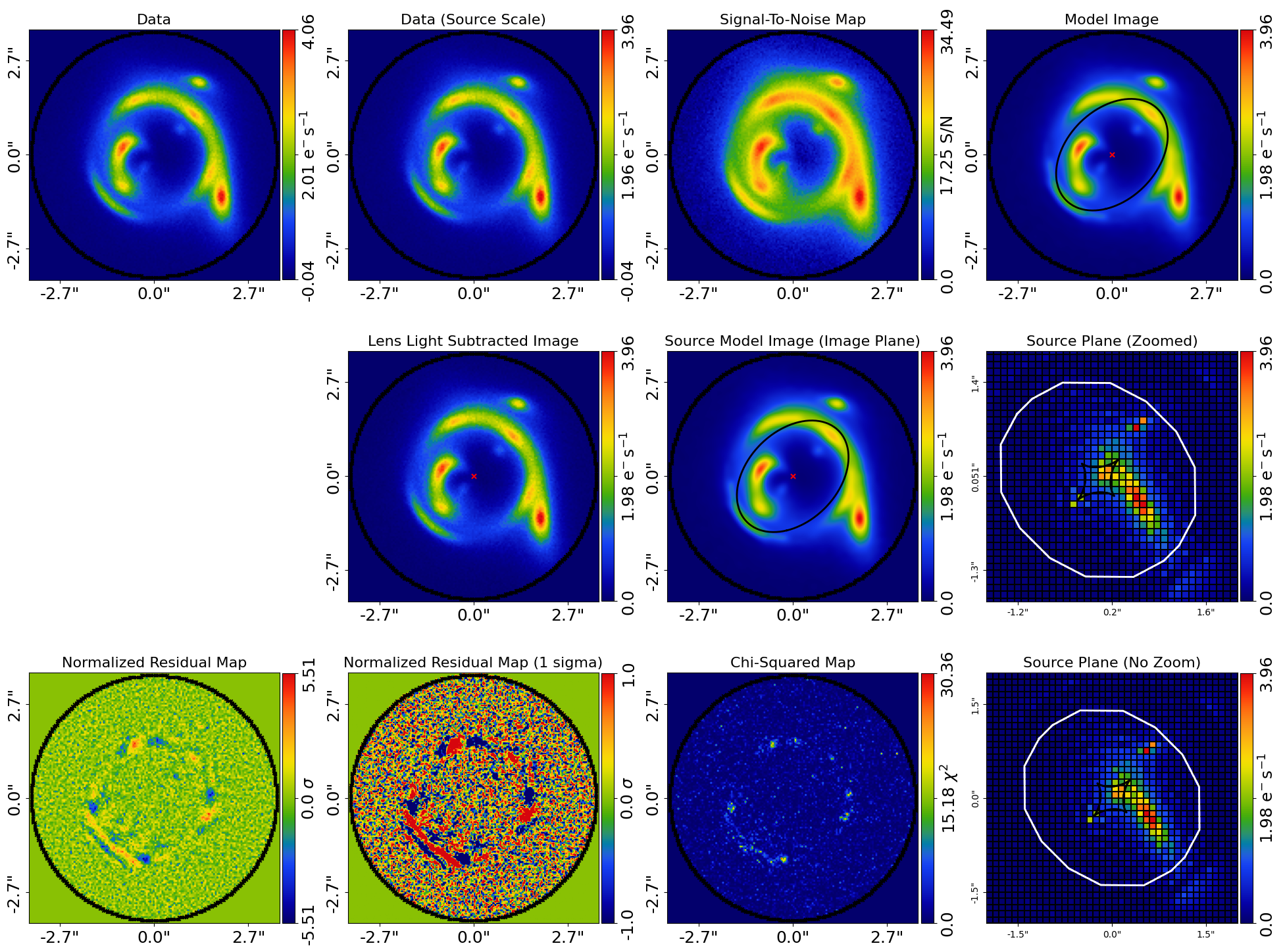
Here is what the subplot looks like, with the following worth noting:
The central-right and bottom-right panel shows a pixelized grid of the subplot show the source has been reconstructed on an uniform rectangular grid of pixels.
The source reconstruction is irregular and has multiple clumps of light, these features would be difficult to represent using analytic light profiles!
The source reconstruction has been mapped back to the image-plane, to produce the reconstructed model image, which is how a
log_likelihoodis computed.This reconstructed model image produces significant residuals, because a rectangular mesh is not an optimal way to reconstruct the source galaxy.
Positive Only Solver#
All pixelized source reconstructions use a positive-only solver, meaning that every source-pixel is only allowed to reconstruct positive flux values. This ensures that the source reconstruction is physical and that we don’t reconstruct negative flux values that don’t exist in the real source galaxy (a common systematic solution in lens analysis).
It may be surprising to hear that this is a feature worth pointing out, but it turns out setting up the linear algebra to enforce positive reconstructions is difficult to make efficient. A lot of development time went into making this possible, where a bespoke fast non-negative linear solver was developed to achieve this.
Other methods in the literature often do not use a positive only solver, and therefore suffer from these unphysical solutions, which can degrade the results of lens model in general.
Alternative Pixelizations#
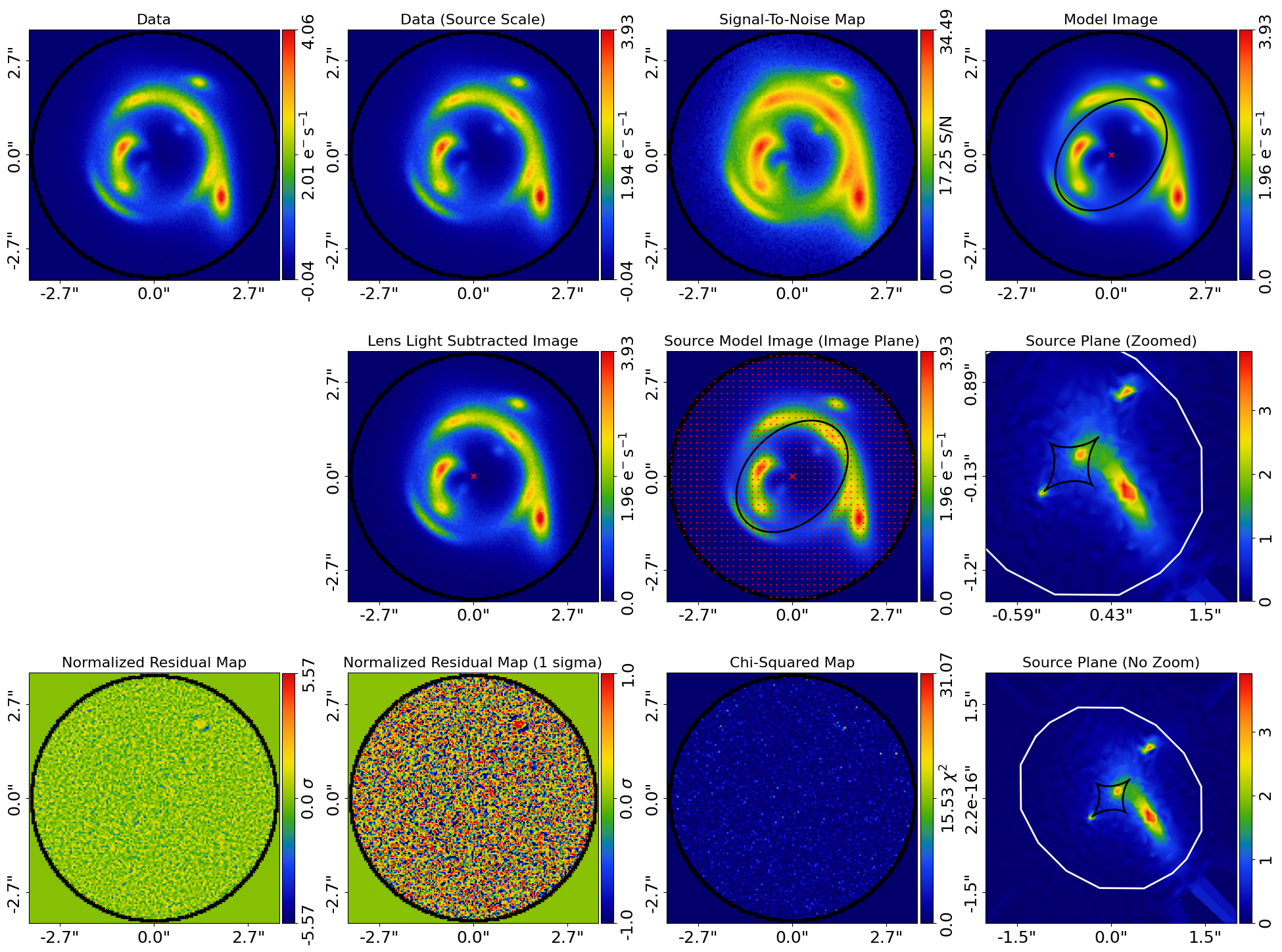
PyAutoLens supports many different meshes. Below, we use a DelaunayMagnification mesh, which defines
the source-pixel centres in the image-plane and ray traces them to the source-plane.
The source pixel-grid is therefore adapted to the mass-model magnification pattern, placing more source-pixel in the highly magnified regions of the source-plane.
This leads to a noticeable improvement in the fit, where the residuals are reduced and the source-reconstruction is noticeably smoother.
pixelization = al.Pixelization(
    mesh=al.mesh.DelaunayMagnification(shape=(40, 40)),
    regularization=al.reg.Constant(coefficient=1.0),
)

source_galaxy = al.Galaxy(redshift=1.0, pixelization=pixelization)

tracer = al.Tracer(galaxies=[lens_galaxy, source_galaxy])

fit = al.FitImaging(dataset=dataset, tracer=tracer)

fit_plotter = aplt.FitImagingPlotter(fit=fit)
fit_plotter.subplot_fit()
Here is the subplot:
Voronoi#
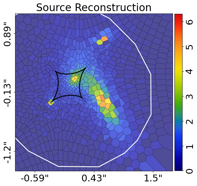
The pixelization mesh which tests have revealed performs best is the VoronoiNN object, which uses a Voronoi
mesh with a technique called natural neighbour interpolation (full details are provided in the HowToLens
tutorials).
I recommend users use this pixelization, how it requires a c library to be installed, thus it is not the default pixelization used in this tutorial.
If you want to use this pixelization, checkout the installation instructions here:
https://github.com/Jammy2211/PyAutoArray/tree/main/autoarray/util/nn
Here is an example of a source reconstruction using this pixelization:
Wrap-Up#
This script has given a brief overview of pixelizations.
A full descriptions of this feature, including an example of how to use pixelizations in lens modeling,
is given in the pixelization example:
In chapter 4 of the HowToLens lectures we fully cover all aspects of using pixelizations, including:
How the source reconstruction determines the flux-values of the source it reconstructs.
The Bayesian framework employed to choose the appropriate level of regularization and avoid overfitting noise.
Unphysical lens model solutions that often arise when using pixelizations
Advanced pixelizations that adapt their properties (e.g. the source pixel locations) to the source galaxy being reconstructed.