Lensing

When two galaxies are aligned perfectly down the line-of-sight to Earth, the background galaxy’s light is bent by the intervening mass of the foreground galaxy. Its light can be fully bent around the foreground galaxy, traversing multiple paths to the Earth, meaning that the background galaxy is observed multiple times. This by-chance alignment of two galaxies is called a strong gravitational lens and a two-dimensional scheme of such a system is pictured below.

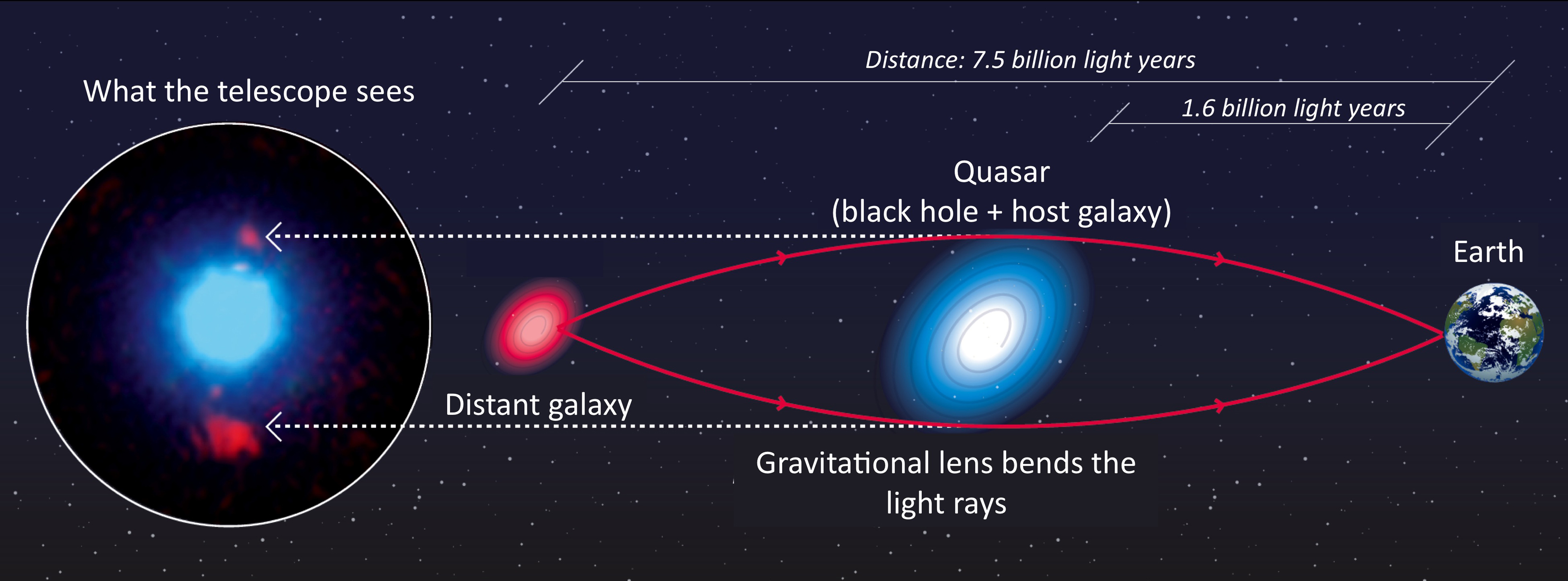
(Image Credit: Image credit: F. Courbin, S. G. Djorgovski, G. Meylan, et al., Caltech / EPFL / WMKO, https://www.astro.caltech.edu/~george/qsolens/)

PyAutoLens is software for analysing strong lenses!

To use PyAutoLens we first import autolens and the plot module.

import autolens as al
import autolens.plot as aplt

Grids

To describe the deflection of light due to the lens galaxy’s mass, PyAutoLens uses Grid2D data structures, which are two-dimensional Cartesian grids of (y,x) coordinates.

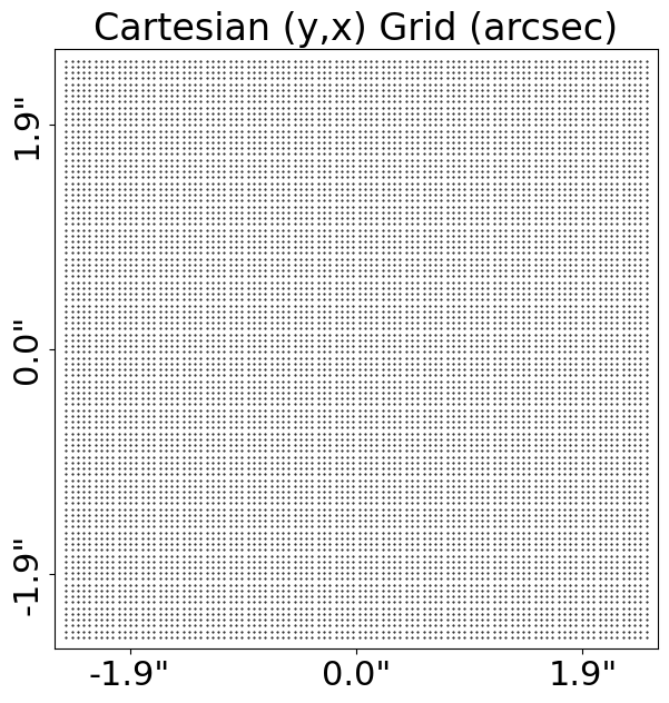
Below, we create and plot a uniform Cartesian Grid2D in units of arcseconds (the pixel_scales describes the conversion from pixel units to arc-seconds).

All quantities which are distance units (e.g. coordinate centre’s radii) are in units of arc-seconds, as this is the most convenient unit to represent lensing quantities:

grid = al.Grid2D.uniform(
    shape_native=(50, 50), pixel_scales=0.05
)
grid_plotter = aplt.Grid2DPlotter(grid=grid)
grid_plotter.set_title(label="Cartesian (y,x) Grid (arcsec)")
grid_plotter.figure_2d()

This is what our Grid2D looks like:

Light Profiles

We will ray-trace this Grid2D’s (y,x) coordinates to calculate how a lens galaxy’s mass deflects the source galaxy’s light.

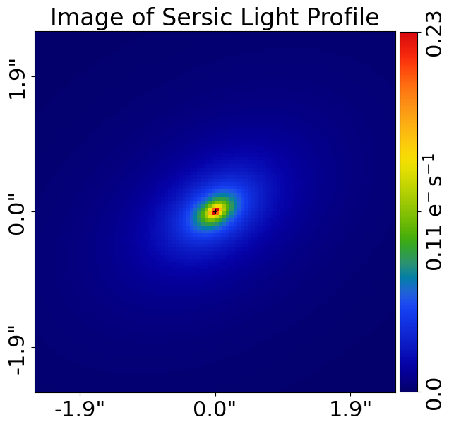
This requires analytic functions representing the light and mass distributions of galaxies, for example the elliptical Sersic LightProfile:

sersic_light_profile = al.lp.Sersic(
    centre=(0.0, 0.0),
    ell_comps=(0.1, 0.1),
    intensity=0.05,
    effective_radius=2.0,
    sersic_index=4.0,
)

By passing this profile a Grid2D, we can evaluate the light at every (y,x) coordinate on the Grid2D and create an image of the Sersic.

All images in PyAutoLens are in units of electrons per second.

image = sersic_light_profile.image_2d_from(grid=grid)

The PyAutoLens plot module provides methods for plotting objects and their properties, like light profile’s image.

light_profile_plotter = aplt.LightProfilePlotter(
    light_profile=sersic_light_profile, grid=grid
)
light_profile_plotter.set_title(label="Image of Sersic Light Profile")
light_profile_plotter.figures_2d(image=True)

The light profile’s image appears as shown below:

Mass Profiles

PyAutoLens uses MassProfile objects to represent a galaxy’s mass distribution and perform ray-tracing calculations.

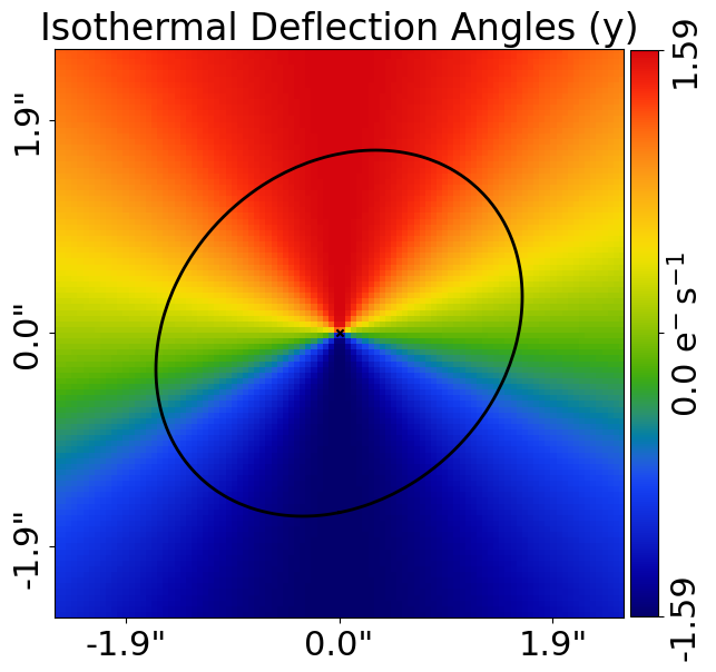
Below we create an Isothermal mass profile and compute its deflection angles on our Cartesian grid, which describe how light rays are deflected as they pass this mass distribution.

isothermal_mass_profile = al.mp.Isothermal(
    centre=(0.0, 0.0), ell_comps=(0.1, 0.0), einstein_radius=1.6
)
deflections = isothermal_mass_profile.deflections_yx_2d_from(grid=grid)

We can plot the isothermal mass profile’s deflection angle map.

The black curve on the figure is the tangential critical curve of the mass profile, if you do not know what this is don’t worry about it for now!

mass_profile_plotter = aplt.MassProfilePlotter(
    mass_profile=isothermal_mass_profile, grid=grid
)
mass_profile_plotter.set_title(label="Isothermal Mass Deflection-Angles (y)")
mass_profile_plotter.figures_2d(
    deflections_y=True,
)
mass_profile_plotter.set_title(label="Isothermal Mass Deflection-Angles (x)")
mass_profile_plotter.figures_2d(
    deflections_x=True,
)

Here is what they look like:

mass_profile_plotter.set_title(label="Isothermal Mass Convergence")
mass_profile_plotter.figures_2d(
    convergence=True,
)
mass_profile_plotter.set_title(label="Isothermal Mass Potential")
mass_profile_plotter.figures_2d(
    potential=True,
)

Here is what they look like:

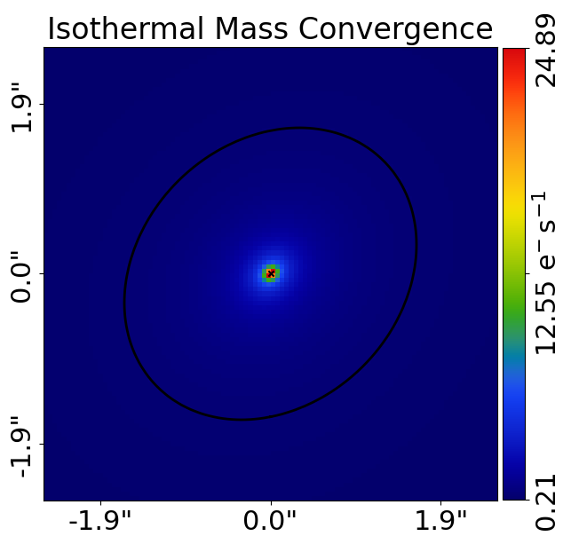
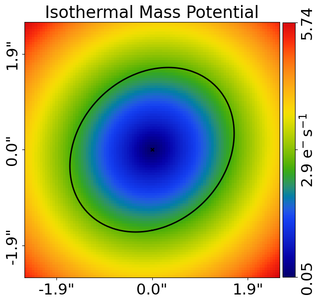
If you are not familiar with gravitational lensing and therefore are unclear on what the convergence and potential are, don’t worry for now!

Galaxies

A Galaxy object is a collection of LightProfile and MassProfile objects at a given redshift. The code below creates two galaxies representing the lens and source galaxies shown in the strong lensing diagram above.

lens_galaxy = al.Galaxy(
    redshift=0.5, bulge=sersic_light_profile, mass=isothermal_mass_profile
)

source_light_profile = al.lp.Exponential(
    centre=(0.3, 0.2), ell_comps=(0.1, 0.0), intensity=0.1, effective_radius=0.5
)

source_galaxy = al.Galaxy(redshift=1.0, bulge=source_light_profile)

The geometry of the strong lens system depends on the cosmological distances between the Earth, the lens galaxy and the source galaxy. It therefore depends on the redshifts of the Galaxy objects.

By passing these Galaxy objects to a Tracer, PyAutoLens uses these galaxy redshifts and a cosmological model to create the appropriate strong lens system.

tracer = al.Tracer.from_galaxies(
    galaxies=[lens_galaxy, source_galaxy], cosmology=al.cosmo.Planck15()
)

Ray Tracing

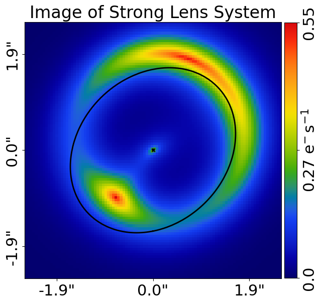
We can now create the image of the strong lens system!

When calculating this image, the Tracer performs all ray-tracing for the strong lens system. This includes using the lens galaxy’s total mass distribution to deflect the light-rays that are traced to the source galaxy. As a result, the source appears as a multiply imaged and strongly lensed Einstein ring.

image = tracer.image_2d_from(grid=grid)

tracer_plotter = aplt.TracerPlotter(tracer=tracer, grid=grid)
tracer_plotter.set_title(label="Image of Strong Lens System")
tracer_plotter.figures_2d(image=True)

This makes the image below, where the source’s light appears as a multiply imaged and strongly lensed Einstein ring.

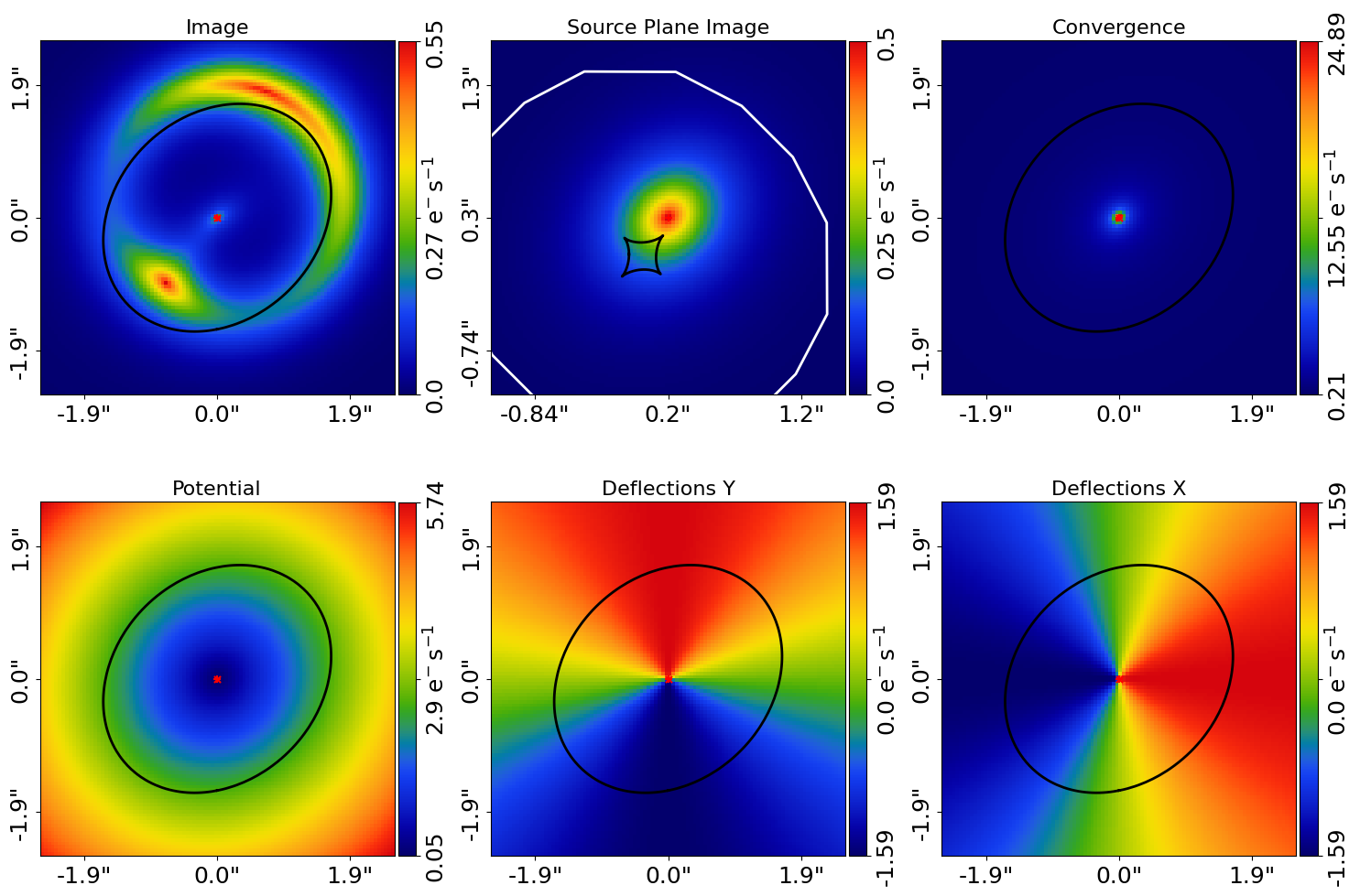
The TracerPlotter includes the MassProfile quantities we plotted previously, which can be plotted as a subplot that plots all these quantities simultaneously.

The black and white lines in the source-plane image are the tangential and radial caustics of the mass, which again you do not need to worry about for now if you don’t know what that is!

tracer_plotter.subplot_tracer()

Here is how the subplot appears:

The tracer is composed of planes. The system above has two planes, an image-plane (at redshift=0.5) and a source-plane (at redshift=1.0).

When creating an image via a Tracer, the mass profiles are used to ray-trace the image-plane grid (plotted above) to a source-plane grid, via the mass profile’s deflection angles.

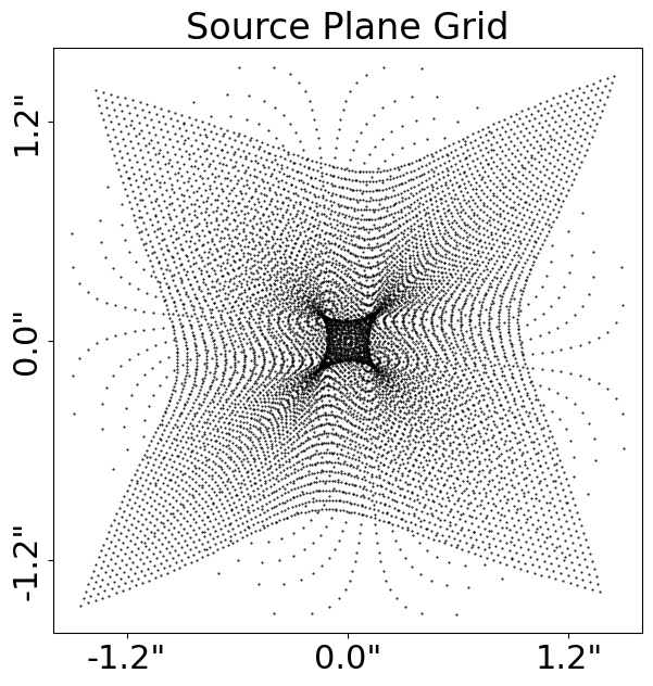
We can use the tracer’s traced_grid_2d_list_from method to calculate and plot the image-plane and source-plane grids.

traced_grid_list = tracer.traced_grid_2d_list_from(grid=grid)

grid_plotter = aplt.Grid2DPlotter(grid=traced_grid_list[0])
grid_plotter.set_title(label="Image-plane Grid")
grid_plotter.figure_2d()

grid_plotter = aplt.Grid2DPlotter(grid=traced_grid_list[1])
grid_plotter.set_title(label="Source-plane Grid")
grid_plotter.figure_2d()  # Source-plane grid.

Here is how they appear:

Extending Objects

The PyAutoLens API has been designed such that all of the objects introduced above are extensible. Galaxy objects can take many LightProfile’s and MassProfile’s. Tracer’ objects can take many Galaxy’s.

If the galaxies are at different redshifts a strong lensing system with multiple lens planes will be created, performing complex multi-plane ray-tracing calculations.

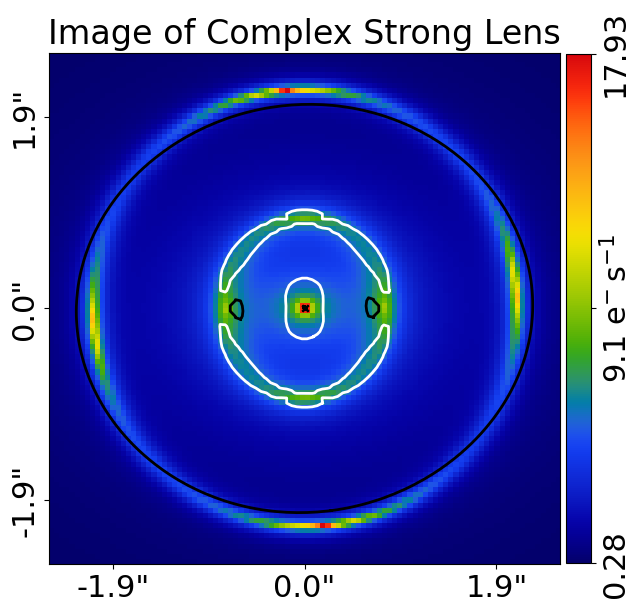
To finish, lets create a Tracer with 3 galaxies at 3 different redshifts, forming a system with two distinct Einstein rings! The mass distribution of the first galaxy also has separate components for its stellar mass and dark matter.

lens_galaxy_0 = al.Galaxy(
    redshift=0.5,
    bulge=al.lmp.Sersic(
        centre=(0.0, 0.0),
        ell_comps=(0.0, 0.05),
        intensity=0.5,
        effective_radius=0.3,
        sersic_index=3.5,
        mass_to_light_ratio=0.6,
    ),
    disk=al.lmp.Exponential(
        centre=(0.0, 0.0),
        ell_comps=(0.0, 0.1),
        intensity=1.0,
        effective_radius=2.0,
        mass_to_light_ratio=0.2,
    ),
    dark=al.mp.NFWSph(centre=(0.0, 0.0), kappa_s=0.08, scale_radius=30.0),
)

lens_galaxy_1 = al.Galaxy(
    redshift=1.0,
    bulge=al.lp.Exponential(
        centre=(0.00, 0.00),
        ell_comps=(0.05, 0.05),
        intensity=1.2,
        effective_radius=0.1,
    ),
    mass=al.mp.Isothermal(
        centre=(0.0, 0.0), ell_comps=(0.05, 0.05), einstein_radius=0.3
    ),
)

source_galaxy = al.Galaxy(
    redshift=2.0,
    bulge=al.lp.Sersic(
        centre=(0.0, 0.0),
        ell_comps=(0.0, 0.111111),
        intensity=1.4,
        effective_radius=0.1,
        sersic_index=1.5,
    ),
)

tracer = al.Tracer.from_galaxies(galaxies=[lens_galaxy_0, lens_galaxy_1, source_galaxy])
tracer_plotter = aplt.TracerPlotter(tracer=tracer, grid=grid)
tracer_plotter.set_title(label="Image of Complex Strong Lens System")
tracer_plotter.figures_2d(image=True)

This is what the lens looks like.

Note how crazy the critical curves are!

Wrap Up

If you are unfamiliar with strong lensing and not clear what some of the above quantities or plots mean, fear not, in chapter 1 of the HowToLens lecture series we’ll take you through strong lensing theory in detail, whilst teaching you how to use PyAutoLens at the same time!

Checkout the tutorials section of the readthedocs!