Features#
This page provides an overview of the advanced features of PyAutoLens.
Firstly, brief one sentence descriptions of each feature are given, with more detailed descriptions below including links to the relevant workspace examples.
Pixelizations: Reconstructing the source galaxy on a mesh of pixels, to capture extremely irregular structures like spiral arms.
Point Sources: Modeling point sources (e.g. quasars) observed in the strong lens imaging data.
Interferometry: Modeling of interferometer data (e.g. ALMA, LOFAR) directly in the uv-plane.
Data Cubes: Modeling spectral-line data cubes (e.g. ALMA CO cubes), fitting every channel simultaneously with a shared lens model.
Multi Gaussian Expansion (MGE): Decomposing the lens galaxy into hundreds of Gaussians, for a clean lens subtraction.
Groups: Modeling group-scale strong lenses with multiple lens galaxies and multiple source galaxies.
Multi-Wavelength: Simultaneous analysis of imaging and / or interferometer datasets observed at different wavelengths.
Ellipse Fitting: Fitting ellipses to determine a lens galaxy’s ellipticity, position angle and centre.
Shapelets: Decomposing a galaxy into a set of shapelet orthogonal basis functions, capturing more complex structures than simple light profiles.
Operated Light Profiles: Assuming a light profile has already been convolved with the PSF, for when the PSF is a significant effect.
Sky Background: Including the background sky in the model to ensure robust fits to the outskirts of galaxies.
Pixelizations#
Pixelizations reconstruct the source galaxy’s light on a pixel-grid. Unlike LightProfile’s, they are able to
reconstruct the light of non-symmetric, irregular and clumpy sources.
The image below shows a pixelized source reconstruction of the strong lens SLACS1430+4105, where the source is reconstructed on a Voronoi mesh adapted to the source morphology, revealing it to be a grand-design face on spiral galaxy:

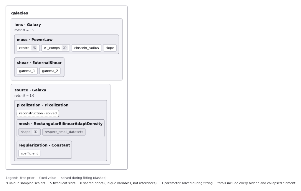
The lens model a pixelized source composes is drawn below: the source’s only sampled parameter is its
regularization coefficient, while the reconstruction — the surface brightness of every source pixel — is solved
for during the fit.
A complete overview of pixelized source reconstructions can be found
at notebooks/overview/overview_5_pixelizations.ipynb.
Chapter 3 of the HowToLens lectures describes pixelizations in detail and teaches users how they can be used to perform lens modeling.
Point Sources#
There are many lenses where the background source is not extended but is instead a point-source, for example strongly lensed quasars and supernovae.
For these objects, we do not want to model the source using a light profile, which implicitly assumes an extended surface brightness distribution.
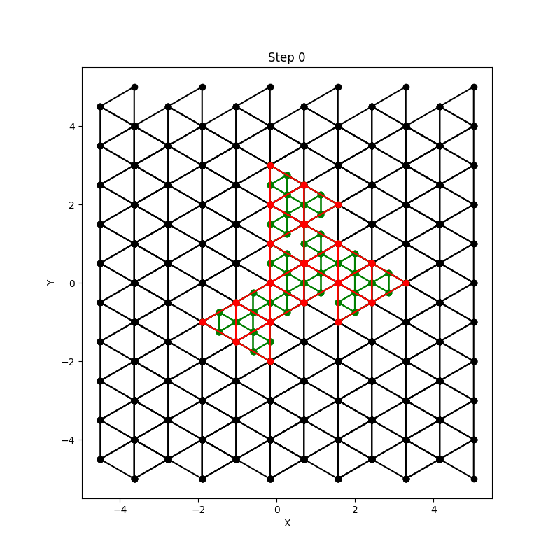
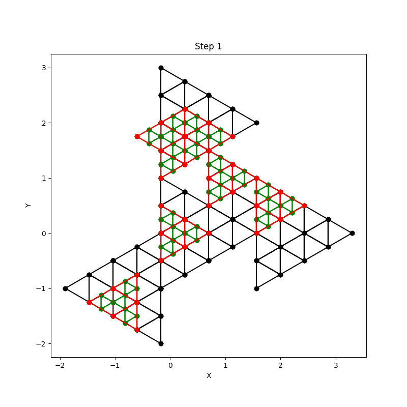
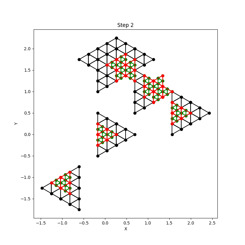
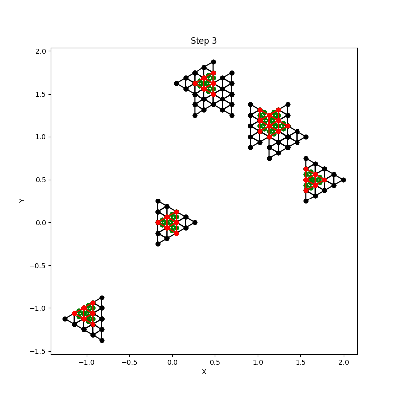
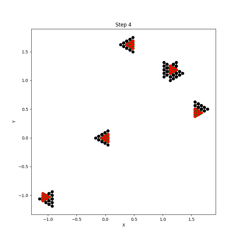
Instead, we assume that our source is a point source with a centre (y,x), and ray-trace triangles at iteratively higher resolutions to determine the source’s exact locations in the image-plane:
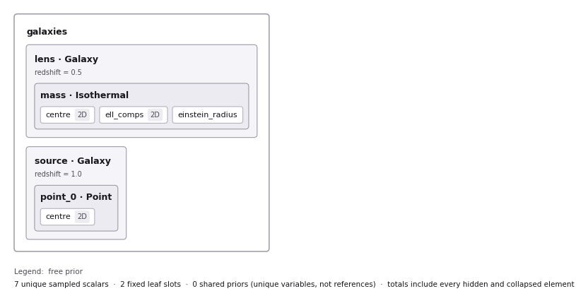
The lens model this composes is drawn below: the source galaxy carries a single al.ps.Point component whose
centre is a sampled two-dimensional parameter. (Using al.ps.PointSolved instead solves that centre analytically
rather than sampling it.)
Note that the image positions above include the fifth central image of the strong lens, which is often not seen in strong lens imaging data. It is easy to disable this image in the point source modeling.
Checkout the autolens_workspace/*/point_source package to get started.
Interferometry#
Modeling of interferometer data from submillimeter (e.g. ALMA) and radio (e.g. LOFAR) observatories:
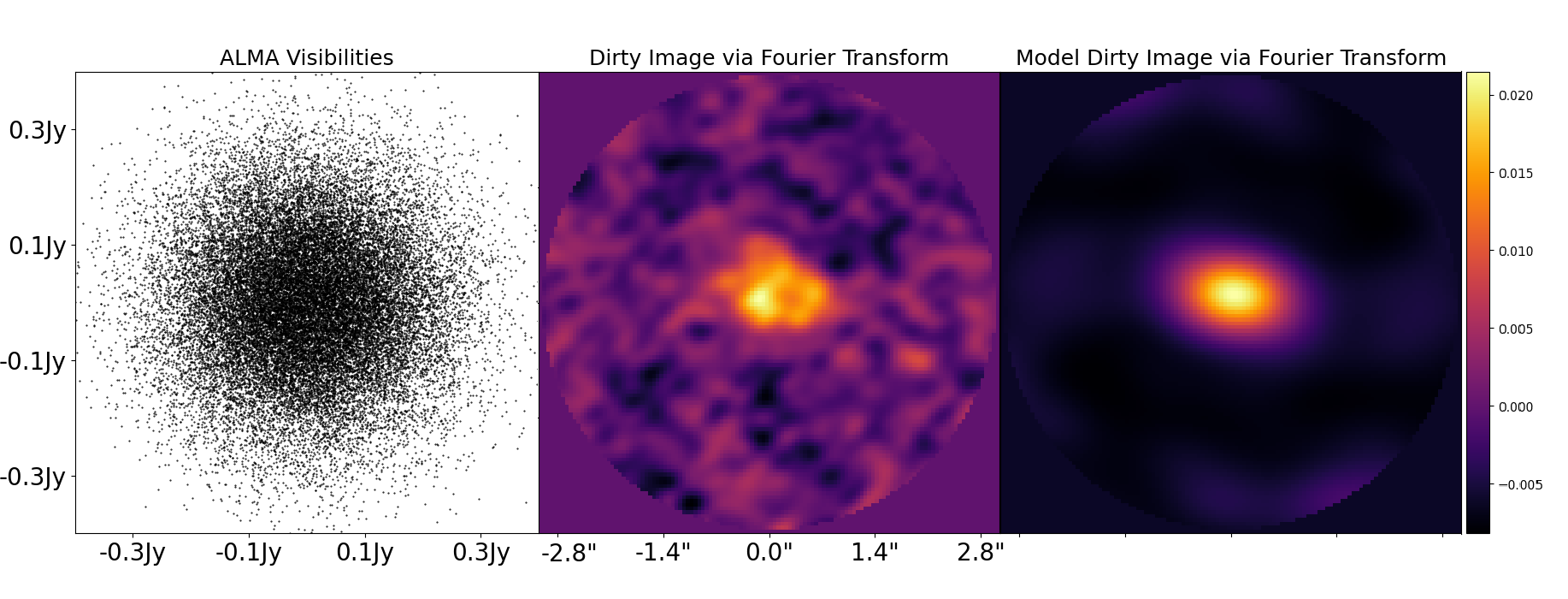
Visibilities data is fitted directly in the uv-plane, circumventing issues that arise when fitting a dirty image such as correlated noise. This uses the non-uniform fast fourier transform algorithm [nufftax](https://github.com/GragasLab/nufftax) to efficiently map the galaxy model images to the uv-plane.
Checkout the autolens_workspace/*/interferometer package to get started.
Data Cubes#
Spectral-line observations produce a data cube: the same field observed in many adjacent frequency channels, so that the source’s emission-line kinematics can be studied alongside the lens model.
A cube is modeled as a list of Interferometer datasets, one per channel, combined into a single fit with
af.FactorGraphModel. Every channel shares one lens mass model, while each channel reconstructs its own source, so
the lens is constrained by the whole cube simultaneously rather than channel by channel. There is no separate cube
dataset type to learn — the existing Interferometer and AnalysisInterferometer objects are reused throughout.
Channel-invariant quantities (the lensing operator’s curvature matrix) are computed once and shared across channels rather than rebuilt per channel, which is what makes fitting a many-channel cube tractable.
Checkout the autolens_workspace/*/interferometer/features/datacube package to get started, which includes a
data_preparation example covering the conversion from a CASA-style 4D FITS cube to the inputs the fit expects.
Multi Gaussian Expansion (MGE)#
An MGE decomposes the light of a galaxy into tens or hundreds of two dimensional Gaussians:
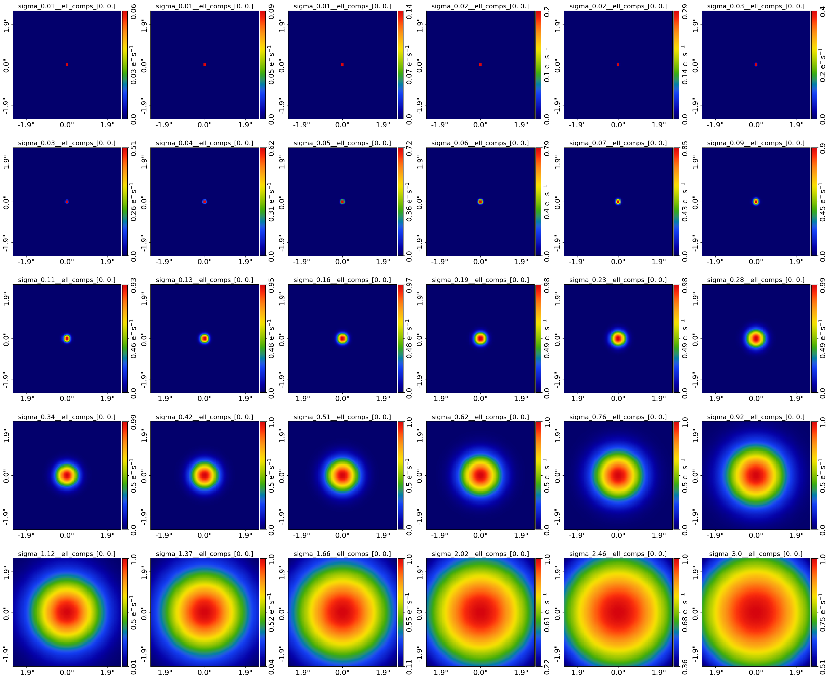
In the image above, 30 Gaussians are shown, where their sizes go from below the pixel scale (in order to resolve point emission) to beyond the size of the galaxy (to capture its extended emission).
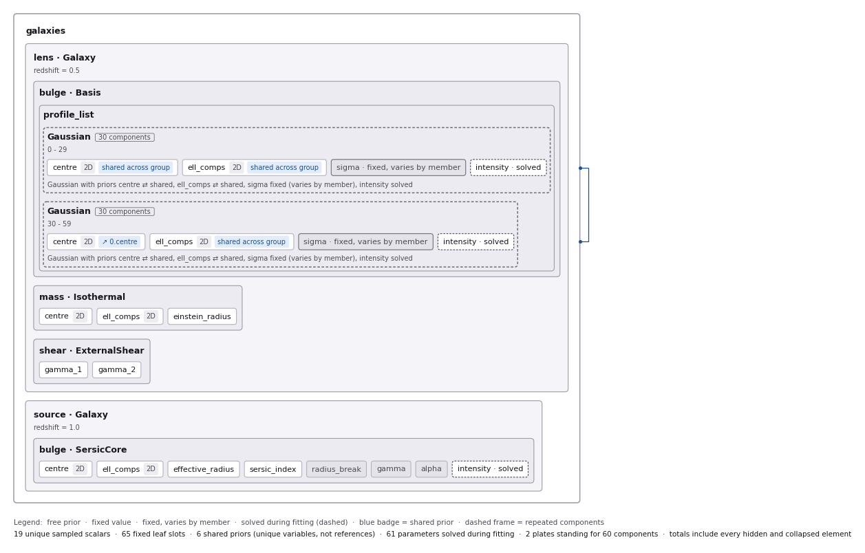
The lens model this composes is drawn below. It is built from two bases of 30 Gaussians each, whose intensity
parameters are solved for by the inversion rather than sampled.
An MGE is an extremely powerful way to model and subtract the light of the foreground lens galaxy in strong lens imaging, and makes it possible to model the stellar mass of the lens galaxy in a way that is tied to its light.
Scientific Applications include capturing departures from elliptical symmetry in the light of galaxies, providing a flexible model to deblend the emission of point sources (e.g. quasars) from the emission of their host galaxy and deprojecting the light of a galaxy from 2D to 3D.
The following paper gives a detailed overview of MGEs and their applications in strong lensing: https://arxiv.org/abs/2403.16253
Checkout autolens_workspace/notebooks/features/multi_gaussian_expansion.ipynb to learn how to use an MGE.
Multi-Galaxy Lenses, Groups and Clusters#
The strong lenses we’ve discussed so far have just a single lens galaxy responsible for the lensing. Above that
scale, PyAutoLens organises lenses into a ladder of three regimes (see the New User Guide for the full
routing): multi-galaxy lenses have two or more co-dominant lens galaxies and no shared dark-matter halo
(autolens_workspace/*/multi_galaxy); group-scale lenses add a group dark-matter halo as an explicit modelling
choice, with fainter members on scaling relations; and cluster-scale lenses keep the group’s mass framework but
switch the analysis to point-source multiple-image positions of many sources. The image below shows a group-scale
system, where multiple lens galaxies deflect one or more background sources:
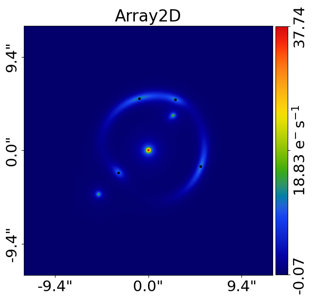
PyAutoLens has built in tools for modeling group-scale lenses, with no limit on the number of lens and source galaxies!
Overviews of group and analysis are given in notebooks/overview/overview_9_groups.ipynb
The autolens_workspace/*/group package has example scripts for simulating datasets and lens modeling.
Multi-Wavelength#
Modeling imaging datasets observed at different wavelengths (e.g. HST F814W and F150W) simultaneously or simultaneously analysing imaging and interferometer data:


The appearance of the strong changes as a function of wavelength, therefore multi-wavelength analysis means we can learn more about the different components in a galaxy (e.g a redder bulge and bluer disk) or when imaging and interferometer data are combined, we can compare the emission from stars and dust.
Checkout the autolens_workspace/*/multi_dataset package to get started, however combining datasets is a more advanced
feature and it is recommended you first get to grips with the core API.
Ellipse Fitting#
Ellipse fitting is a technique which fits many ellipses to a galaxy’s emission to determine its ellipticity, position angle and centre, without assuming a parametric form for its light (e.g. like a Seisc profile):
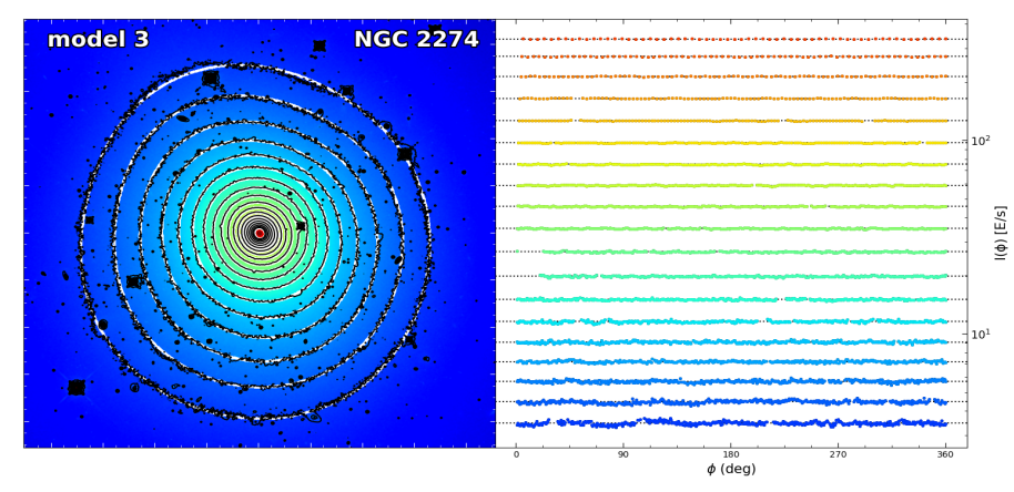
This provides complementary information to parametric light profile fitting, for example giving insights on whether the ellipticity and position angle are constant with radius or if the galaxy’s emission is lopsided.
There are also multipole moment extensions to ellipse fitting, which determine higher order deviations from elliptical symmetry providing even more information on the galaxy’s structure.
The following paper describes the technique in detail: https://arxiv.org/html/2407.12983v1
Checkout autolens_workspace/notebooks/features/ellipse_fitting.ipynb to learn how to use ellipse fitting.
Shapelets#
Shapelets are a set of orthogonal basis functions that can be combined the represent galaxy structures:
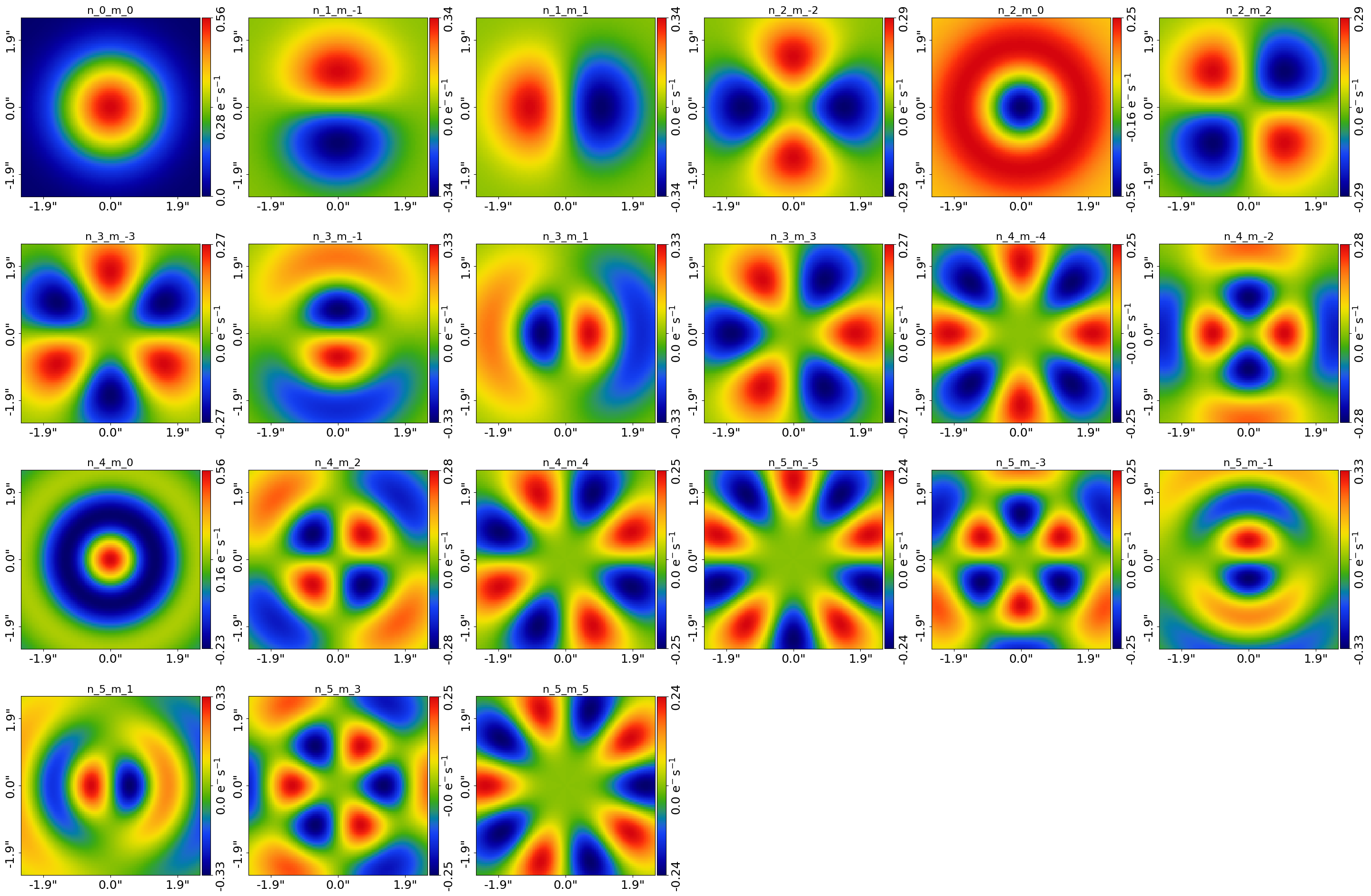
Scientific Applications include capturing symmetric structures in a galaxy which are more complex than a Sersic profile, irregular and asymmetric structures in a galaxy like spiral arms and providing a flexible model to deblend the emission of point sources (e.g. quasars) from the emission of their host galaxy.
Checkout autolens_workspace/notebooks/features/shapelets.ipynb to learn how to use shapelets.
Operated Light Profiles#
An operated light profile is one where it is assumed to already be convolved with the PSF of the data, with the
Moffat and Gaussian profiles common choices:
They are used for certain scientific applications where the PSF convolution is known to be a significant effect and the knowledge of the PSF allows for detailed modeling abd deblending of the galaxy’s light.
Checkout autogalaxy_workspace/notebooks/features/operated_light_profiles.ipynb to learn how to use operated profiles.
Sky Background#
When an image of a galaxy is observed, the background sky contributes light to the image and adds noise:
For detailed studies of the outskirts of galaxies (e.g. stellar halos, faint extended disks), the sky background must be accounted for in the model to ensure robust and accurate fits.
Checkout autogalaxy_workspace/notebooks/features/sky_background.ipynb to learn how to use include the sky
background in your model.
Mass Models#
The examples above model the lens’s mass with an isothermal profile, but PyAutoLens supports a wide range of mass models:
Total mass profiles (e.g. the isothermal and power-law) represent the combined stellar and dark matter mass of the lens galaxy with a single profile. Decomposed mass models fit the stellar and dark matter separately, tying the stellar mass to the light (e.g. via an MGE) and adding an NFW dark matter halo, directly measuring the balance of stellar and dark matter in the galaxy.
Multipole perturbations (m=1, m=3 and m=4) extend any mass model with departures from elliptical symmetry, capturing lopsidedness, boxiness / disciness and bar-like structures in the mass distribution. Accounting for this angular complexity is critical for many science cases, as unmodeled angular structure can masquerade as other signals, for example dark matter substructure.
The following paper measures angular mass complexity alongside dark matter substructure in JWST strong lens imaging: https://arxiv.org/abs/2410.12987
The role of the m=1 multipole (lopsidedness) is detailed in: https://arxiv.org/abs/2407.12983
Checkout autolens_workspace/*/guides/profiles for the full range of mass profiles
and autolens_workspace/*/imaging/features/advanced/mass_stellar_dark for decomposed stellar + dark matter
modeling.
Automated Pipelines / SLaM#
Fitting complex lens models (e.g. a decomposed mass model with a pixelized source) in one non-linear search is often infeasible: the parameter space is too complex for the fit to converge reliably or efficiently.
Search chaining breaks the fit into a sequence of simpler searches, where the results of each search initialize the model of the next. The Source, Light and Mass (SLaM) pipelines are PyAutoLens’s pre-built implementation of this approach: they first build a robust model of the source, then the lens’s light, and finally its mass, gradually increasing model complexity. The SLaM pipelines have been used in many published PyAutoLens analyses and are the recommended way to perform detailed lens modeling of large samples.
Checkout autolens_workspace/*/guides/modeling/slam_start_here.py to get started with the SLaM pipelines.
Dark Matter Subhalos#
The dark matter model predicts that galaxies are surrounded by many low-mass dark matter subhalos, which host no stars and are therefore invisible to ordinary observations. Strong lensing is one of the only probes which can detect them, via the small perturbations they imprint on a lensed source’s light, testing the nature of dark matter (e.g. cold, warm or self-interacting).
PyAutoLens provides a complete dark matter subhalo analysis: lens models with and without a subhalo are fitted and compared via their Bayesian evidence, quantifying whether the data favors the subhalo’s presence. Sensitivity mapping then simulates subhalos of different masses at different locations in the data, quantifying which subhalos a given dataset could actually detect.
The following paper performs this analysis on a sample of HST strong lenses: https://arxiv.org/abs/2209.10566
Checkout autolens_workspace/*/imaging/features/advanced/subhalo/detect for subhalo detection
and autolens_workspace/*/imaging/features/advanced/subhalo/sensitivity for sensitivity mapping.
Graphical Models#
The examples above fit each strong lens dataset one-by-one. However, many lens properties are shared across a sample (e.g. population-level mass distributions, cosmological parameters), and fitting lenses independently does not exploit this shared structure.
Graphical models fit multiple datasets simultaneously, explicitly defining which parameters are unique to each lens and which are shared across the sample. For example, the Hubble constant can be inferred jointly from many time-delay lenses, with each lens having its own mass model but all sharing a single H0. Hierarchical extensions assume parameters are drawn from a parent distribution (e.g. the population’s distribution of mass slopes), whose properties are inferred from the full sample, extracting significantly more information than one-by-one fitting.
Checkout autolens_workspace/*/guides/modeling/advanced/graphical.py to learn how to fit a graphical model
and autolens_workspace/*/guides/modeling/advanced/hierarchical.py for hierarchical models.
Weak Lensing#
In the weak lensing regime, a foreground mass distribution (e.g. a galaxy cluster) subtly distorts the shapes of many background galaxies, coherently aligning their ellipticities, without producing the multiple images and giant arcs of strong lensing.
PyAutoLens fits weak lensing shear catalogues using the same mass profiles and non-linear search tools as strong lensing: model-independent mass maps, parametric halo model fits and tangential shear profiles. Its quickstart example fits the real JWST-era shape catalogue of Abell 2744, and strong and weak lensing data can be combined in joint analyses of the same cluster.
Checkout autolens_workspace/*/weak/start_here.py to fit your first weak lensing dataset.