Start Here#

PyAutoLens is software for analysing strong gravitational lenses, an astrophysical phenomenon where a galaxy appears multiple times because its light is bent by the gravitational field of an intervening foreground lens galaxy.

Here is a schematic of a strong gravitational lens:

Alternative text

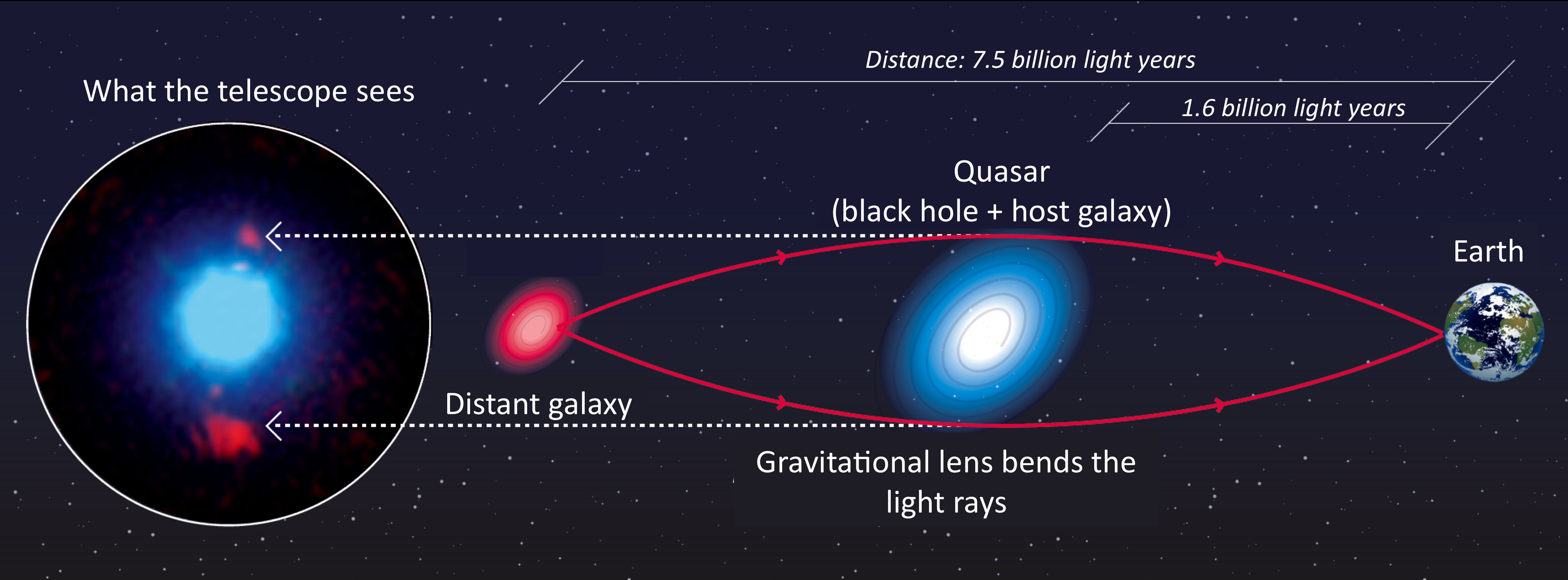
Credit: F. Courbin, S. G. Djorgovski, G. Meylan, et al., Caltech / EPFL / WMKO https://www.astro.caltech.edu/~george/qsolens/

This notebook gives an overview of PyAutoLens’s features and API.

Imports#

Lets first import autolens, its plotting module and the other libraries we’ll need.

You’ll see these imports in the majority of workspace examples.

import autolens as al
import autolens.plot as aplt

import matplotlib.pyplot as plt
from os import path

Lets illustrate a simple gravitational lensing calculation, creating an an image of a lensed galaxy using a light profile and mass profile.

Grid#

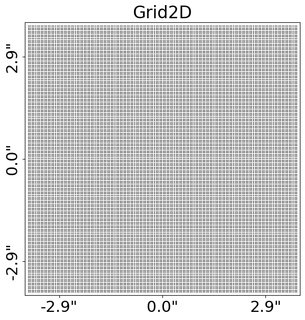
The emission of light from a source galaxy, which is gravitationally lensed around the lens galaxy, is described using the Grid2D data structure, which is two-dimensional Cartesian grids of (y,x) coordinates.

We make and plot a uniform Cartesian grid:

grid = al.Grid2D.uniform(
    shape_native=(150, 150),  # The [pixels x pixels] shape of the grid in 2D.
    pixel_scales=0.05,  # The pixel-scale describes the conversion from pixel units to arc-seconds.
)

grid_plotter = aplt.Grid2DPlotter(grid=grid)
grid_plotter.figure_2d()

The Grid2D looks like this:

Alternative text

Light Profiles#

Our aim is to create an image of the source galaxy after its light has been deflected by the mass of the foreground lens galaxy. We therefore need to ray-trace the Grid2D’s coordinates from the ‘image-plane’ to the ‘source-plane’.

This uses analytic functions representing a galaxy’s light and mass distributions, referred to as LightProfile and MassProfile objects.

The most common light profile in Astronomy is the elliptical Sersic, which we create an instance of below:

sersic_light_profile = al.lp.Sersic(
    centre=(0.0, 0.0),  # The light profile centre [units of arc-seconds].
    ell_comps=(
        0.2,
        0.1,
    ),  # The light profile elliptical components [can be converted to axis-ratio and position angle].
    intensity=0.005,  # The overall intensity normalisation [units arbitrary and are matched to the data].
    effective_radius=2.0,  # The effective radius containing half the profile's total luminosity [units of arc-seconds].
    sersic_index=4.0,  # Describes the profile's shape [higher value -> more concentrated profile].
)

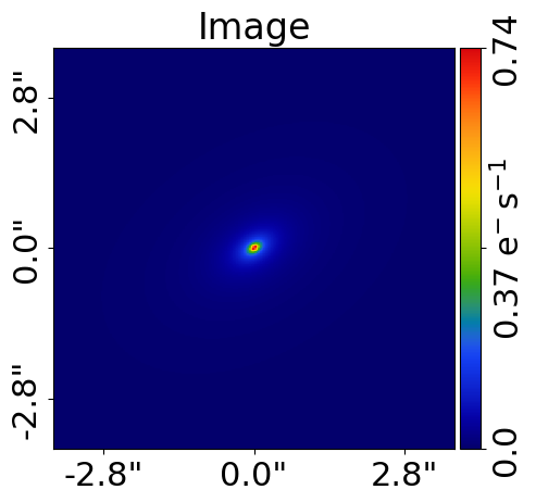
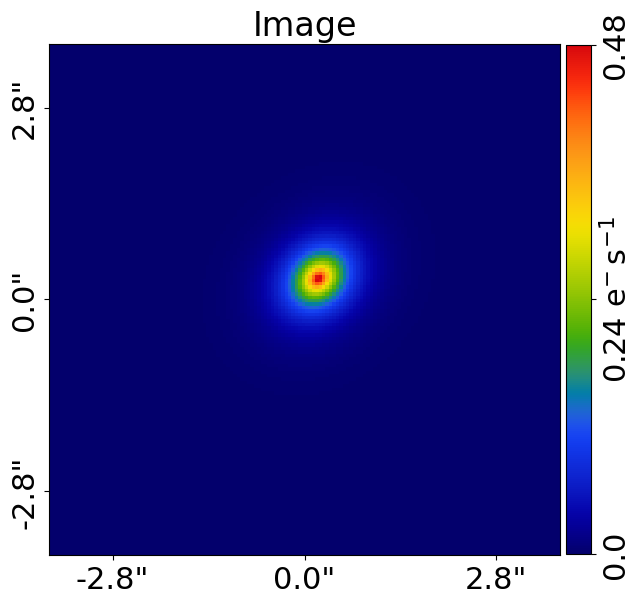
By passing the light profile the grid, we evaluate the light emitted at every (y,x) coordinate and therefore create an image of the Sersic light profile.

image = sersic_light_profile.image_2d_from(grid=grid)

Plotting#

The PyAutoLens in-built plot module provides methods for plotting objects and their properties, like the image of a light profile we just created.

By using a LightProfilePlotter to plot the light profile’s image, the figured is improved.

Its axis units are scaled to arc-seconds, a color-bar is added, its given a descriptive labels, etc.

The plot module is highly customizable and designed to make it straight forward to create clean and informative figures for fits to large datasets.

light_profile_plotter = aplt.LightProfilePlotter(
    light_profile=sersic_light_profile, grid=grid
)
light_profile_plotter.figures_2d(image=True)
Alternative text

Mass Profiles#

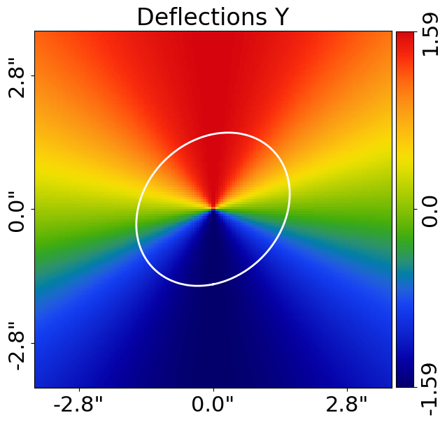
PyAutoLens uses MassProfile objects to represent a galaxy’s mass distribution and perform ray-tracing calculations.

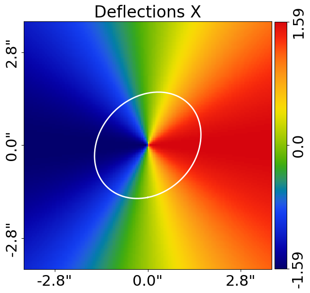
Below we create an elliptical isothermal MassProfile and compute its deflection angles on our Cartesian grid, where the deflection angles describe how the lens galaxy’s mass bends the source’s light:

isothermal_mass_profile = al.mp.Isothermal(
    centre=(0.0, 0.0),  # The mass profile centre [units of arc-seconds].
    ell_comps=(
        0.1,
        0.0,
    ),  # The mass profile elliptical components [can be converted to axis-ratio and position angle].
    einstein_radius=1.6,  # The Einstein radius [units of arc-seconds].
)

deflections = isothermal_mass_profile.deflections_yx_2d_from(grid=grid)

The deflection angles are easily plotted using the PyAutoLens plot module.

(Many other lensing quantities are also easily plotted, for example the convergence and potential).

mass_profile_plotter = aplt.MassProfilePlotter(
    mass_profile=isothermal_mass_profile, grid=grid
)
mass_profile_plotter.figures_2d(
    deflections_y=True,
    deflections_x=True,
    # convergence=True,
    # potential=True
)
Alternative text Alternative text

Galaxy#

A Galaxy object is a collection of light profiles at a specific redshift.

This object is highly extensible and is what ultimately allows us to fit complex models to strong lens images.

Below, we create two galaxies representing the lens and source galaxies shown in the strong lensing diagram above.

lens_galaxy = al.Galaxy(
    redshift=0.5,
    light=sersic_light_profile,  # The foreground lens's light is typically observed in a strong lens.
    mass=isothermal_mass_profile,  # Its mass is what causes the strong lensing effect.
)

source_light_profile = al.lp.Exponential(
    centre=(
        0.3,
        0.2,
    ),  # The source galaxy's light is observed, appearing as multiple images around the lens galaxy.
    ell_comps=(
        0.1,
        0.0,
    ),  # However, the mass of the source does not impact the strong lensing effect.
    intensity=0.1,  # and is not included.
    effective_radius=0.5,
)

source_galaxy = al.Galaxy(redshift=1.0, light=source_light_profile)

The GalaxyPlotter object plots properties of the lens and source galaxies.

lens_galaxy_plotter = aplt.GalaxyPlotter(galaxy=lens_galaxy, grid=grid)
lens_galaxy_plotter.figures_2d(image=True, deflections_y=True, deflections_x=True)

source_galaxy_plotter = aplt.GalaxyPlotter(galaxy=source_galaxy, grid=grid)
source_galaxy_plotter.figures_2d(image=True)
Alternative text Alternative text Alternative text Alternative text

One example of the plotter’s customizability is the ability to plot the individual light profiles of the galaxy on a subplot.

lens_galaxy_plotter.subplot_of_light_profiles(image=True)
Alternative text

Tracer#

The Tracer object is the most important object in PyAutoLens.

It is a collection of galaxies at different redshifts (often referred to as planes).

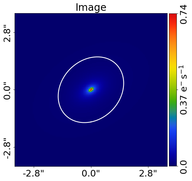
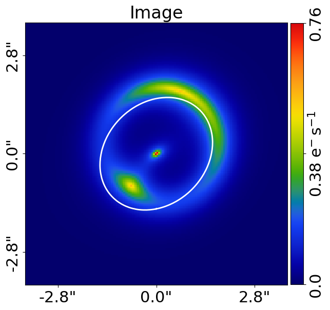
It uses these galaxies to perform ray-tracing, using the mass profiles of the galaxies to bend the light of the source galaxy(s) into the multiple images we observe in a strong lens system.

This is shown below, where the image of the tracer shows a distinct Einstein ring of the source galaxy.

tracer = al.Tracer(galaxies=[lens_galaxy, source_galaxy], cosmology=al.cosmo.Planck15())

image = tracer.image_2d_from(grid=grid)

tracer_plotter = aplt.TracerPlotter(tracer=tracer, grid=grid)
tracer_plotter.figures_2d(image=True)
Alternative text

Units#

The units used throughout the strong lensing literature vary, therefore lets quickly describe the units used in PyAutoLens.

The Tracer object and all mass profiles describe their quantities in terms of angles, which are defined in units of arc-seconds. To convert these to physical units (e.g. kiloparsecs), we use the redshift of the lens and source galaxies and an input cosmology. A run through of all normal unit conversions is given in guides in the workspace that are discussed later.

The use of angles in arc-seconds has an important property, it means that for a two-plane strong lens system (e.g. a lens galaxy at one redshift and source galaxy at another redshift) lensing calculations are independent of the galaxies’ redshifts and the input cosmology. This has a number of benefits, for example it makes it straight forward to compare the lensing properties of different strong lens systems even when the redshifts of the galaxies are unknown.

Multi-plane lensing is when there are more than two planes. The tracer fully supports this, if you input 3+ galaxies with different redshifts into the tracer it will use their redshifts and its cosmology to perform multi-plane lensing calculations that depend on them.

Extensibility#

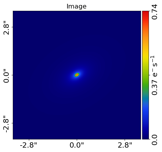
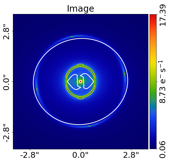
All of the objects we’ve introduced so far are highly extensible, for example a tracer can be made of many galaxies, a galaxy can be made up of any number of light profiles and many galaxy objects can be combined into a galaxies object.

Below, wecreate a Tracer with 3 galaxies at 3 different redshifts, forming a system with two distinct Einstein rings! The mass distribution of the first galaxy has separate components for its stellar mass and dark matter, where the stellar components use a LightAndMassProfile via the lmp module.

lens_galaxy_0 = al.Galaxy(
    redshift=0.5,
    bulge=al.lmp.Sersic(
        centre=(0.0, 0.0),
        ell_comps=(0.0, 0.05),
        intensity=0.5,
        effective_radius=0.3,
        sersic_index=3.5,
        mass_to_light_ratio=0.6,
    ),
    disk=al.lmp.Exponential(
        centre=(0.0, 0.0),
        ell_comps=(0.0, 0.1),
        intensity=1.0,
        effective_radius=2.0,
        mass_to_light_ratio=0.2,
    ),
    dark=al.mp.NFWSph(centre=(0.0, 0.0), kappa_s=0.08, scale_radius=30.0),
)

lens_galaxy_1 = al.Galaxy(
    redshift=1.0,
    bulge=al.lp.Exponential(
        centre=(0.00, 0.00),
        ell_comps=(0.05, 0.05),
        intensity=1.2,
        effective_radius=0.1,
    ),
    mass=al.mp.Isothermal(
        centre=(0.0, 0.0), ell_comps=(0.05, 0.05), einstein_radius=0.6
    ),
)

source_galaxy = al.Galaxy(
    redshift=2.0,
    bulge=al.lp.Sersic(
        centre=(0.0, 0.0),
        ell_comps=(0.0, 0.111111),
        intensity=0.7,
        effective_radius=0.1,
        sersic_index=1.5,
    ),
)

tracer = al.Tracer(galaxies=[lens_galaxy_0, lens_galaxy_1, source_galaxy])

tracer_plotter = aplt.TracerPlotter(tracer=tracer, grid=grid)
tracer_plotter.figures_2d(image=True)
Alternative text

Simulating Data#

The strong lens images above are not what we would observe if we looked at the sky through a telescope.

In reality, images of strong lenses are observed using a telescope and detector, for example a CCD Imaging device attached to the Hubble Space Telescope.

To make images that look like realistic Astronomy data, we must account for the effects like how the length of the exposure time change the signal-to-noise, how the optics of the telescope blur the galaxy’s light and that there is a background sky which also contributes light to the image and adds noise.

The SimulatorImaging object simulates this process, creating realistic CCD images of galaxies using the Imaging object.

simulator = al.SimulatorImaging(
    exposure_time=300.0,
    background_sky_level=1.0,
    psf=al.Kernel2D.from_gaussian(shape_native=(11, 11), sigma=0.1, pixel_scales=0.05),
    add_poisson_noise_to_data=True,
)

Once we have a simulator, we can use it to create an imaging dataset which consists of an image, noise-map and Point Spread Function (PSF) by passing it a galaxies and grid.

This uses the tracer above to create the image of the galaxy and then add the effects that occur during data acquisition.

This data is used below to illustrate model-fitting, so lets simulate a very simple image of a strong lens.

lens_galaxy = al.Galaxy(
    redshift=0.5,
    light=al.lp.Sersic(
        centre=(0.0, 0.0),
        ell_comps=(
            0.2,
            0.1,
        ),
        intensity=0.005,
        effective_radius=2.0,
        sersic_index=4.0,
    ),
    mass=al.mp.Isothermal(centre=(0.0, 0.0), ell_comps=(0.1, 0.0), einstein_radius=1.6),
)

source_galaxy = al.Galaxy(
    redshift=1.0,
    light=al.lp.Exponential(
        centre=(0.3, 0.2), ell_comps=(0.1, 0.0), intensity=0.1, effective_radius=0.5
    ),
)

tracer = al.Tracer(galaxies=[lens_galaxy, source_galaxy], cosmology=al.cosmo.Planck15())

dataset = simulator.via_tracer_from(tracer=tracer, grid=grid)

Observed Dataset#

We now have an Imaging object, which is a realistic representation of the data we observe with a telescope.

We use the ImagingPlotter to plot the dataset, showing that it contains the observed image, but also other import dataset attributes like the noise-map and PSF.

dataset_plotter = aplt.ImagingPlotter(dataset=dataset)
dataset_plotter.figures_2d(data=True)
Alternative text

If you have come to PyAutoLens to perform interferometry, the API above is easily adapted to use a SimulatorInterferometer object to simulate an Interferometer dataset instead.

However, you should finish reading this notebook before moving on to the interferometry examples, to get a full overview of the core PyAutoLens API.

Masking#

We are about to fit the data with a model, but first must define a mask, which defines the regions of the image that are used to fit the data and which regions are not.

We create a Mask2D object which is a 3.0” circle, whereby all pixels within this 3.0” circle are used in the model-fit and all pixels outside are omitted.

Inspection of the dataset above shows that no signal from the strong lens is observed outside of this radius, so this is a sensible mask.

mask = al.Mask2D.circular(
    shape_native=dataset.shape_native,  # The mask's shape must match the dataset's to be applied to it.
    pixel_scales=dataset.pixel_scales,  # It must also have the same pixel scales.
    radius=3.0,  # The mask's circular radius [units of arc-seconds].
)

Combine the imaging dataset with the mask.

dataset = dataset.apply_mask(mask=mask)

When we plot a masked dataset, the removed regions of the image (e.g. outside the 3.0”) are automatically set to zero and the plot axis automatically zooms in around the mask.

dataset_plotter = aplt.ImagingPlotter(dataset=dataset)
dataset_plotter.figures_2d(data=True)
Alternative text

Fitting#

We are now at the point a scientist would be after observing a strong lens - we have an image of it, have used to a mask to determine where we observe signal from the galaxy, but cannot make any quantitative statements about its mass or source morphology.

We therefore must now fit a model to the data. This model is a representation of the lens galaxy’s light and mass and source galaxy’s light. We seek a way to determine whether a given model provides a good fit to the data.

A fit is performing using a FitImaging object, which takes a dataset and tracer object as input and determine if the galaxies are a good fit to the data.

fit = al.FitImaging(dataset=dataset, tracer=tracer)

The fit creates model_data, which is the image of the strong lens including effects which change its appearance during data acquisition.

For example, by plotting the fit’s model_data and comparing it to the image of the strong lens obtained via the TracerPlotter, we can see the model data has been blurred by the dataset’s PSF.

tracer_plotter = aplt.TracerPlotter(tracer=fit.tracer, grid=grid)
tracer_plotter.figures_2d(image=True)

fit_plotter = aplt.FitImagingPlotter(fit=fit)
fit_plotter.figures_2d(model_image=True)
Alternative text Alternative text

The fit also creates the following:

  • The residual_map: The model_image subtracted from the observed dataset``s image.

  • The normalized_residual_map: The residual_map ``divided by the observed dataset's ``noise_map.

  • The chi_squared_map: The normalized_residual_map squared.

We can plot all 3 of these on a subplot that also includes the data, signal-to-noise map and model data.

In this example, the tracer used to simulate the data are used to fit it, thus the fit is good and residuals are minimized.

fit_plotter.subplot_fit()

The overall quality of the fit is quantified with the log_likelihood.

print(fit.log_likelihood)

If you are familiar with statistical analysis, this quick run-through of the fitting tools will make sense and you will be familiar with concepts like model data, residuals and a likelihood.

If you are less familiar with these concepts, I recommend you finish this notebook and then go to the fitting API guide, which explains the concepts in more detail and provides a more thorough overview of the fitting tools.

The take home point is that PyAutoLens’s API has extensive tools for fitting models to data and visualizing the results, which is what makes it a powerful tool for studying the morphologies of galaxies.

Modeling#

The fitting tools above are used to fit a model to the data given an input set of galaxies. Above, we used the true galaxies used to simulate the data to fit the data, but we do not know what this “truth” is in the real world and is therefore not something a real scientist can do.

Modeling is the processing of taking a dataset and inferring the model that best fits the data, for example the galaxy light and mass profile(s) that best fits the light observed in the data or equivalently the combination of Sersic profile parameters that maximize the likelihood of the fit.

Lens modeling uses the probabilistic programming language PyAutoFit, an open-source project that allows complex model fitting techniques to be straightforwardly integrated into scientific modeling software. Check it out if you are interested in developing your own software to perform advanced model-fitting:

https://github.com/rhayes777/PyAutoFit

We import PyAutoFit separately to PyAutoLens:

import autofit as af

We now compose the galaxy model using af.Model objects.

These behave analogously to the Galaxy, LightProfile and MassProfile objects above, however their parameters are not specified and are instead determined by a fitting procedure.

We will fit our galaxy data with a model which has one galaxy where:

We will fit our strong lens data with two galaxies:

  • A lens galaxy with a Sersic LightProfile representing its light and an Isothermal MassProfile representing its mass.

  • A source galaxy with an Exponential LightProfile representing a disk.

The redshifts of the lens (z=0.155) and source(z=0.517) are fixed, but as discussed above their values do not matter for a two-plane lens system because the units of angles in arc-seconds are independent of the redshifts.

The light profiles below are linear light profiles, input via the lp_linear module. These solve for the intensity of the light profiles via linear algebra, making the modeling more efficient and accurate. They are explained in more detail in other workspace examples, but are a key reason why modeling with PyAutoLens performs well and can scale to complex models.

galaxy_model = af.Model(
    al.Galaxy,
    redshift=0.5,
    bulge=al.lp_linear.Sersic,
    disk=al.lp_linear.Exponential,
)

lens = af.Model(
    al.Galaxy,
    redshift=0.155,
    bulge=al.lp_linear.Sersic,  # Note the use of ``lp_linear`` instead of ``lp``.
    mass=al.mp.Isothermal,  # This uses linear light profiles explained in the modeling ``start_here`` example.
)

source = af.Model(al.Galaxy, redshift=0.517, disk=al.lp_linear.Exponential)

We combine the lens and source model galaxies above into a Collection, which is the model we will fit.

Note how we could easily extend this object to compose highly complex models containing many galaxies.

model = af.Collection(galaxies=af.Collection(lens=lens, source=source))

By printing the Model’s we see that each parameters has a prior associated with it, which is used by the model-fitting procedure to fit the model.

print(model)

The info attribute shows the model information in a more readable format:

print(model.info)

We now choose the ‘non-linear search’, which is the fitting method used to determine the light profile parameters that best-fit the data.

In this example we use [nautilus](https://nautilus-sampler.readthedocs.io/en/stable/), a nested sampling algorithm that in our experience has proven very effective at galaxy modeling.

search = af.Nautilus(name="start_here")

To perform the model-fit, we create an AnalysisImaging object which contains the log_likelihood_function that the non-linear search calls to fit the galaxy model to the data.

The AnalysisImaging object is expanded on in the modeling start_here example, but in brief performs many useful associated with modeling, including outputting results to hard-disk and visualizing the results of the fit.

analysis = al.AnalysisImaging(dataset=dataset)

To perform the model-fit we pass the model and analysis to the search’s fit method. This will output results (e.g., Nautilus samples, model parameters, visualization) to your computer’s storage device.

However, the lens modeling of this system takes a minute or so. Therefore, to save time, we have commented out the fit function below so you can skip through to the next section of the notebook. Feel free to uncomment the code and run the galaxy modeling yourself!

Once a model-fit is running, PyAutoLens outputs the results of the search to storage device on-the-fly. This includes galaxy model parameter estimates with errors non-linear samples and the visualization of the best-fit galaxy model inferred by the search so far.

result = search.fit(model=model, analysis=analysis)

The animation below shows a slide-show of the lens modeling procedure. Many lens models are fitted to the data over and over, gradually improving the quality of the fit to the data and looking more and more like the observed image.

We can see that initial models give a poor fit to the data but gradually improve (increasing the likelihood) as more iterations are performed.

https://github.com/Jammy2211/auto_files/blob/main/lensmodel.gif?raw=true

![Lens Modeling Animation](https://github.com/Jammy2211/auto_files/blob/main/lensmodel.gif?raw=true “model”)

Credit: Amy Etherington

Results#

The fit returns a Result object, which contains the best-fit galaxies and the full posterior information of the non-linear search, including all parameter samples, log likelihood values and tools to compute the errors on the galaxy model.

Using results is explained in full in the guides/results section of the workspace, but for a quick illustration the commented out code below shows how easy it is to plot the fit and posterior of the model.

fit_plotter = aplt.FitImagingPlotter(fit=result.max_log_likelihood_fit)
fit_plotter.subplot_fit()

plotter = aplt.NestPlotter(samples=result.samples)
plotter.corner_cornerpy()

Here is an example corner plot of the model-fit, which shows the probability density function of every parameter in the model:

Alternative text

Wrap Up#

We have now completed the API overview of PyAutoLens, including a brief introduction to the core API for creating galaxies, simulating data, fitting data and performing galaxy modeling.

The next overview describes how a new user should navigate the PyAutoLens workspace, which contains many examples and tutorials, in order to get up and running with the software.